Econometric Methodology | RDP 9111: Monthly Movements in the Australian Dollar and Real Short-Term Interest Differentials: An Application of the Kalman Filter

RDP 9111: Monthly Movements in the Australian Dollar and Real Short-Term Interest Differentials: An Application of the Kalman Filter 4. Econometric Methodology

Alison Tarditi and Gordon Menzies

November 1991

Download the Paper 488KB

A state space representation of the structural model is derived to avoid the computational problems arising from the inclusion of unobserved variables. The resulting representation can then be estimated using the Kalman filter. Harvey (1988)^[29] describes this method of model specification and estimation as being “… in many ways preferable to the more conventional approach based on ARIMA processes”. This section briefly reviews Kalman filter estimation and its application in our paper (see Harvey (1981, 1988, and 1989) for a detailed discussion).

4.1 Motivation for Choice of Estimation Technique

The Kalman filter was derived for applications in control engineering (Kalman (1960)). In this paper, its importance for maximum likelihood estimation is exploited. Depending on the form of the function to be optimised, maximum likelihood problems can be solved either analytically or numerically. The analytical solution involves equating the vector of first derivatives to zero and solving for the parameters. More complex functions are solved numerically. Two approaches exist for numerical optimisation:

Direct evaluation is used for functions which can be calculated but not differentiated.
Kalman filter evaluation is used either because the likelihood function cannot be evaluated directly, or because the system contains unobservable variables.

Our paper uses the Kalman filter because it permits a more flexible and rigorous treatment of the unobservable variables, the ex ante real interest differential, E_t(d_t,t+1) the long-run real exchange rate, w_t, and the forecast error, e_t.^[30] The alternative approach, selecting proxy variables before estimation, is subject to measurement error and may not be optimal in any well-defined sense.

The more standard method of estimating models with unobservable components is that of “instrumental variables” (IV). This technique relies on choosing a proxy (or “instrument”) which, while highly correlated with its unobservable equivalent, is not correlated with the model's disturbance terms. The parameter estimates obtained in this way are sensitive to the choice of instrument and may be biased. The IV technique would also restrict the dynamics of Campbell and Clarida's (1987) structural model:

The long-run real equilibrium exchange rate and the risk premium are allowed to vary over time. Determining an instrument for either of these variables is problematic. With respect to wt, a separate model could be estimated, but this exercise lies beyond the scope of our paper. The temptation would be to assume wt constant as in Shafer and Loopesko (1983). Moreover, these assumptions reduce the explanatory power of the model.
We suggest that d_t−1 would be an appropriate instrument for E_t(d_t,t+1).^[31] Using IV, equation [10] could be estimated as:

View MathML

where:

w is a constant term representing the long-run real exchange rate;
ω_t is a composite error term incorporating u_1,t, u_2,t and u_3,t.

Estimation of [10'] reveals strong serial correlation. This can be corrected by using an appropriate estimation technique (for example simple Cochrane-Orcutt AR(1) modification). Alternatively, the model can be estimated in first differences. Although this approach would yield coefficient estimates, it would eliminate evaluation of the proportion of the variation in q_t explained by E_t(d_t,t+1). Rather, it would enable us to evaluate the proportion of the variation in the change in q_t explained by the change in the proxy for E_t(d_t,t+1).

As well, the Kalman filter allows solution of the model regardless of stationary/non-stationary data considerations.

4.2 Application of the Kalman Filter

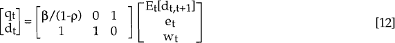
The filter can only be applied once the structural model is cast in a framework which enables the treatment of its unobservable components. A linear dynamic system can be written in the so-called state space form.^[32] A key feature of this representation is the presence of an unobservable vector, α_t called the state vector. In the context of this paper, α_t is [E_t(d_t,t+1) e_t w_t]'.

The state space form consists of two equations: the measurement equation and the transition equation. The measurement equation relates the vector of unobservable, explanatory variables, α_t, to a vector of observable variables, y_t, such that:

For our model this takes the form:

β ≠ 1 : Linear risk premium model;
β = 1 : Uncovered interest parity model;

β and ρ are assumed constant for these two models and, in keeping with our theory-based relationships, an error term – generally added onto the right-hand-side of equation [11] – is not included.

The second equation in the state space formulation is the transition equation. This describes the evolution of the state vector over time such that:

For our model:

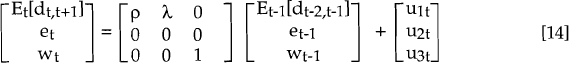
u_1t is the innovation, unrelated to inflation surprise, associated with the ex ante real interest differential. u_2t is the inflation forecast error; rational expectations dictates that this is uncorrelated contemporaneously with either u_1t or u_3t. u_3t is the innovation to the long-run real exchange rate. All errors are serially uncorrelated and have standard deviations σ₁, σ₂ and σ₃ respectively. σ₁₃, the contemporaneous covariance between u_1t and u_3t, is not restricted.

Initialised with a set of priors, the Kalman filter estimates (that is, it “predicts” and “updates”) the vector of unobservable variables, α_t period by period. “Predicting” means predicting α_t given the information set of period t-1. “Updating” means using a one-step-ahead forecast error of y_t (necessarily calculated by the filter at each execution) to update the predicted value of α_t. This two stage procedure, carried out at each new time period, defines the Kalman filter. The linear estimate of α_t denoted , is optimal in the minimum mean square error sense. The filter also provides the error covariance matrix of , denoted P_t. Starting values for and P₀ must be provided. At time period t, observations y₁, y₂ … y_t are available.

Apart from its ability to generate optimal estimates (as opposed to proxies) for the vector of unobservable variables, α_t the Kalman filter may be used in maximum likelihood estimation. Its execution generates a time series for the one-step-ahead prediction errors made in estimating the vector of observable, dependent variables, y_t. Harvey (1985) notes that the likelihood can be calculated from these normally distributed errors and their variances. Estimation of our model yields a bivariate normal log likelihood function which can be expressed as:

where:

υ_t is the set of one-step-ahead prediction errors made in estimating the vector of observable, explanatory variables, y_t (the real exchange rate, q_t, and the ex post real interest differential, d_t, in our model). That is, υ_t = y_t – E_t−1[y_t]. The one-step-ahead prediction of the observation y_t is calculated as: 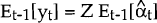where is the optimal predictor of the state vector, α_t, given observations up to t−1 and Z is the matrix of coefficients on the state vector.
F_t is the estimated covariance matrix of these one-step-ahead prediction errors.

Hence, the Kalman filter can be run in conjunction with an optimisation routine^[33] – calculating the likelihood where required by the routine. This is what it means to “estimate” a model using the Kalman filter. For each run through the filter, the coefficients on the model are fixed. However, the likelihood function [15] can be calculated for each run.^[34]

Equations [12] and [14] are estimated with the Kalman filter. The model contains seven unknown parameters, β, ρ, λ, σ₁, σ₂, σ₃ and σ₁₃. Where equality between the expected real exchange rate change and the real interest differential is imposed, β is set equal to one. We estimate models for Australia's real exchange rate with the United States, Japan, West Germany and the United Kingdom, as well as a trade-weighted index. In each case, models are estimated with β unrestricted and with β restricted to one.

4.3 Variance Decomposition

Innovation relationships were investigated by expanding the one-period ahead variance of the actual dependent variable (namely, the observable real exchange rate) in the following manner.

Equation [10] implies:

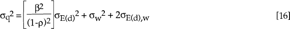
where the subscripts of σ carry their obvious meaning (refer equation [10]).

The variance T periods ahead (i.e., E_t(q_t+T−Et(q_t+T))²) is

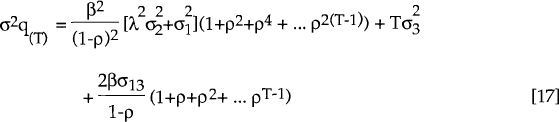
as T →∞, the first and third terms of the RHS converge, i.e.:

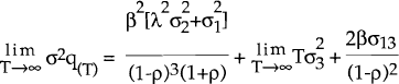
Clearly, a variance decomposition calculated over a long time horizon will always attribute a very large proportion of the variation in q_T to w_t a priori. This is a direct result of the assumption that w_t is a random walk and that E_t(d_t) is stationary. In the limit, w_t explains 100 per cent of the variation in q_T. However, what is not imposed is how much of the variability in q_T is explained by w_t in the short run. In principle, ρ could be very close to one, in which case E_t(d_t,t+1) could explain a large proportion of the variability of q_t for a small value of T. Using the parameter estimates obtained from the Kalman filter and the optimisation algorithm, the appropriate expression for the variance (equation [17] with T=1) is used to calculate estimated variance decompositions. That is, each of the three terms on the right hand side of equation [17] are expressed as a percentage of σ_q(1)² and reported in Tables 4 and 5.

Footnotes

Harvey (1988), Chapter 8, p.285. [29]

Clearly, the specification of the unobservable components in the state space model must depend, to some extent, on a priori considerations. However, estimates of the unobservable variables generated by the Kalman filter are optimal in the minimum MSE sense. [30]

Since the second time-series assumption describes E_t(d_t,t+1) as a stationary AR(1) process, d_t can be shown to follow an ARMA(1,1) process of the form:

(See Fama and Gibbons (1982) for other working to show that if ex ante real interest rates follow a univariate AR(1), then ex post real rates must follow a univariate ARMA (1,1)). The complex error structure of this equation highlights a limitation to the IV approach (given that the error structure proposed by Campbell and Clarida (1987) is a plausible one). Restricting u_1,t to zero transforms this equation into a standard ARMA(1,1) that may be estimated by IV. The resulting estimate of ρ using data for our trade-weighted index is not significantly different from one. In contrast, estimates of p generated by the Kalman filter are 0.59 in the linear risk premium model and 0.62 in the uncovered interest parity model. These estimates accord with those of Gruen and Wilkinson (1991) who, using the augmented Dickey-Fuller test, estimate equivalent coefficients at 0.66.
Nevertheless, given the IV approach to estimation, ρ = 1, and d_t−1 becomes a suitable instrument for E_t(d_t,t+1). [31]

Such models, driven by innovations of some macroeconomic time series, are sometimes referred to as “innovation models” (see Aoki and Havenner (1986)). [32]

Since it is explicitly designed for optimisation of likelihood functions, the Berndt-Hall-Hall-Hausman (1974) algorithm (BHHH) is used on the final iteration for all models, with the exception of the United Kingdom. BHHH uses a modified method of scoring (see Berndt et al. (1974)) to optimise the function. On the final iteration of the United Kingdom's uncovered interest parity model, a more general purpose algorithm is applied. [33]

See Appendix 2 for a flow chart of our estimation procedure. [34]