RDP 9510: Modelling Inflation in Australia Appendix 2: Design of the Empirical ECM
November 1995
- Download the Paper 264KB
This appendix discusses several of the steps taken to obtain the ECM in (17) and examines in greater detail the recursive estimates of the coefficients in (17). This simplification to (17) has numerous motivations. Because of its parsimony and more orthogonal regressors, (17) is more easily interpreted than the unrestricted ADL or VAR. Also, the coefficients in (17) are more precisely estimated than those in the ADL and the VAR, providing tighter inferences generally and higher potential power for tests of mis-specification.
Initially, the vector autoregression for the system cointegration analysis is simplified from a fourth-order VAR to a first-order VAR, where the variables in the VARs are p, ulc, ip, pet, a constant, and centered seasonal dummies. Table A1 reports the F statistics and related calculations for that simplification, where the longest lag on all variables is deleted repeatedly from the VAR. None of the F statistics comparing the initial, intermediate, and final VARs is significant; and the Schwarz criterion becomes steadily more negative as the lag length is shortened. The Schwarz criterion in effect adjusts a measure of the model's goodness of fit (the log of the determinant of the estimated error variance matrix) for the model's degree of parsimony. A smaller Schwarz criterion indicates a better-fitting model for a given number of parameters, or a more parsimonious model for a given goodness of fit.
| Null Hypothesis | Maintained Hypothesis | ||||||
|---|---|---|---|---|---|---|---|
| System | k |  |
SC | VAR(4) | VAR(3) | VAR(2) | |
| VAR(4) | 80 |
1111.5 |
−29.06 |
– – |
|||
| ↓ | – | ||||||
| VAR(3) | 64 |
1101.8 |
−29.79 |
0.82 [0.66] |
|||
| ↓ | (16,128) | ||||||
| VAR(2) | 48 |
1091.0 |
−30.49 |
0.91 [0.61] |
1.02 [0.44] |
||
| ↓ | (32,156) | (16,141) | |||||
| VAR(1) | 32 |
1079.2 |
−31.15 |
1.00 [0.48] |
1.11 [0.32] |
1.21 [0.26] |
|
| (48,163) | (32,171) | (16,153) | |||||
Notes |
|||||||
Having tested for and found weak exogeneity for unit labour costs, import prices, and petrol prices (Table 2), a fourth-order autoregressive distributed lag for the CPI is simplified to the ECM in (17). Table A2 lists the estimates of the coefficients for the fourth-order ADL, where the ADL has been transformed into its unrestricted ECM representation (11). The following variables do not appear either numerically or statistically significant.
| Variable |
Lag i | |||
|---|---|---|---|---|
| 0 | 1 | 2 | 3 | |
| Δpt−i | −1.0 (–) |
−0.063 (0.141) |
0.136 (0.138) |
−0.043 (0.146) |
| Δulct−i | 0.042 (0.031) |
−0.020 (0.028) |
−0.021 (0.029) |
−0.007 (0.028) |
| Δipt−i | 0.021 (0.016) |
−0.011 (0.019) |
−0.003 (0.021) |
0.000 (0.019) |
| Δpett−i | 0.011 (0.007) |
0.006 (0.009) |
0.003 (0.009) |
0.007 (0.008) |
| Δyt−i | −0.020 (0.048) |
−0.039 (0.054) |
−0.009 (0.045) |
−0.022 (0.042) |
| pt−i | −0.098 (0.034) |
|||
| ulct−i | 0.051 (0.028) |
|||
| ipt−i | 0.046 (0.016) |
|||
| pett−i | 0.005 (0.005) |
|||
 |
0.080 (0.027) |
|||
| Dt | 0.011 (0.004) |
|||
| Sit | −0.0087 (0.0288) |
−0.0021 (0.0013) |
−0.0011 (0.0011) |
−0.0022 (0.0012) |
T = 65 [1977(3)–1993(3)] R2 = 0.9016  = 0.268%
dw = 2.04 LMp : F(1, 36) = 0.33 AR : F(5, 31) = 0.50 ARCH : F(4, 28) = 0.25 Normality : χ2 (2) = 0.34 RESET : F(1, 35) = 0.17 |
||||
Notes |
||||
- The third lag on Δp, Δulc, Δip, Δpet, and Δy;
- The second lag on Δp, Δulc, Δip, Δpet, and Δy; and
- The first lag on Δp, Δulc, Δip, Δpet, and Δy.
Three additional sets of reductions are considered:
- The sum of the coefficients on ulct–1, ipt–1, and pett–1 equals the negative of the coefficient on pt–1, i.e., long-run homogeneity in prices is satisfied;
- Δulct and Δipt have zero coefficients; and
- Δyt has a zero coefficient.
Treated sequentially, these six restrictions obtain the following seven models.
| Model 1: | The unrestricted ECM in Table A2. |
| Model 2: | Model 1, excluding the third lag on Δp, Δulc, Δip, Δpet, and Δy. |
| Model 3: | Model 2, excluding the second lag on Δp, Δulc, Δip, Δpet, and Δy. |
| Model 4: | Model 3, excluding the first lag on Δp, Δulc, Δip, Δpet, and Δy. |
| Model 5: | Model 4, imposing long-run price homogeneity. |
| Model 6: | Model 5, excluding Δulct and Δipt. |
| Model 7: | Model 6, excluding Δyt. |
So, for example, Model 2 is Model 1 plus reduction (i); Model 3 is Model 1 plus reductions (i)–(ii); and Model 3 is also Model 2 plus reduction (ii).
Table A3 lists the estimates for Model 4 and shows how little the estimates change from imposing the first three reductions. Table A3 also clarifies how the remaining three restrictions appear reasonable.
| Variable |
Lag i | |||
|---|---|---|---|---|
| 0 | 1 | 2 | 3 | |
| Δpt−i | −1.0 (–) |
|||
| Δulct−i | 0.033 (0.022) |
|||
| Δipt−i | 0.012 (0.013) |
|||
| Δpett−i | 0.010 (0.006) |
|||
| Δyt−i | −0.049 (0.030) |
|||
| pt−i | −0.0884 (0.0136) |
|||
| ulct−i | 0.0404 (0.0143) |
|||
| ipt−i | 0.0417 (0.0055) |
|||
| pett−i | 0.0072 (0.0030) |
|||
 |
0.0641 (0.0124) |
|||
| Dt | 0.0103 (0.0028) |
|||
| Sit | 0.0032 (0.0140) |
−0.0022 (0.0010) |
−0.0007 (0.0009) |
−0.0024 (0.0009) |
T = 65 [1977(3)–1993(3)] R2
= 0.8838  = 0.244% = 0.244%dw = 2.13 LMp : F(1, 51) = 0.09 AR : F(5, 46) = 0.27 ARCH : F(4, 43) = 0.95 Normality : χ2 (2) = 1.19 RESET : F(1, 50) = 1.00 Hetero : F(22, 28) = 0.92 |
||||
Notes |
||||
To facilitate formally assessing whether or not the sequence of reductions (i)–(vi) is
valid, and if not, where not, statistics associated with the implied reductions are calculated
for all model pairs, and not only for adjacent models. Table A4 reports this information,
including the estimated equation standard error  and the Schwarz
criterion for each model, the F statistics for all model pairs, and the associated tail
probability values. The equation standard error is relatively constant across the entire
simplification path; and the Schwarz criterion declines steadily through Model 6, remaining
virtually unchanged between Model 6 and Model 7. Only that last reduction (excluding Δyt)
is statistically significant at the 5% level; and it is only barely so, and only when considered
by itself and not in conjunction with previous reductions. Appendix
3 develops an alternative model that includes changes in the output gap. Other orderings of
(i)–(vi) generate somewhat different statistics, but those resulting statistics are
unlikely to be highly statistically significant because the reduction of (i)–(vi) as a
whole appears valid, with F(19, 36) = 0.66 and a
p-value of 0.84.
| Null Hypothesis | Maintained Hypothesis (Model Number) | |||||||||
|---|---|---|---|---|---|---|---|---|---|---|
| Model | k |  |
SC | 1 | 2 | 3 | 4 | 5 | 6 | |
| 1 | 29 |
0.268% |
−10.58 |
– – |
||||||
| ↓ (i) | – | |||||||||
| 2 | 24 |
0.255% |
−10.86 |
0.24 [0.94] |
||||||
| ↓ (ii) | (5,36) | |||||||||
| 3 | 19 |
0.250% |
−11.11 |
0.40 [0.94] |
0.62 [0.69] |
|||||
| ↓ (iii) | (10,36) | (5,41) | ||||||||
| 4 | 14 |
0.244% |
−11.37 |
0.43 [0.96] |
0.59 [0.82] |
0.58 [0.71] |
||||
| ↓ (iv) | (15,36) | (10,41) | (5,46) | |||||||
| 5 | 13 |
0.242% |
−11.43 |
0.41 [0.97] |
0.54 [0.86] |
0.50 [0.81] |
0.09 [0.77] |
|||
| ↓ (v) | (16,36) | (11,41) | (6,46) | (1,51) | ||||||
| 6 | 11 |
0.244% |
−11.51 |
0.49 [0.95] |
0.65 [0.80] |
0.70 [0.69] |
0.93 [0.43] |
1.37 [0.26] |
||
| ↓ (vi) | (18,36) | (13,41) | (8,46) | (3,51) | (2,52) | |||||
| 7 | 10 |
0.251% |
−11.50 |
0.66 [0.84] |
0.89 [0.58] |
1.08 [0.39] |
1.78 [0.15] |
2.38 [0.080] |
4.34 [0.042] |
|
| (19,36) | (14,41) | (9,46) | (4,51) | (3,52) | (1,54) | |||||
Notes |
||||||||||
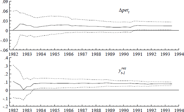
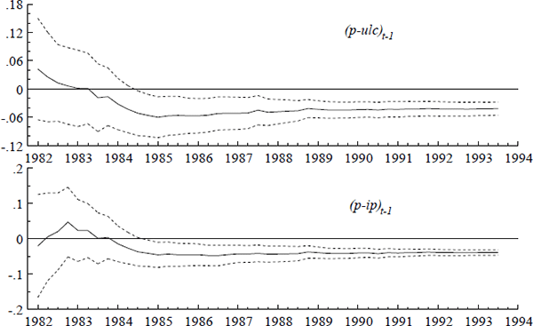
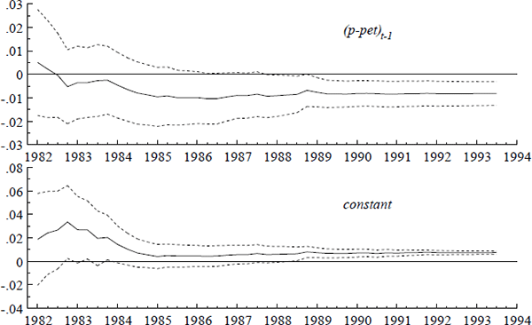
Figures A1–A3 show the recursively estimated coefficients of the economic variables in
(17) and plus-or-minus twice their recursively estimated standard errors, conventionally denoted
 and
and  ± 2ese(
 )
respectively. To provide more interpretable graphs, (17) has been parameterized as (21), in
which all coefficients are unrestricted. Coefficients vary only slightly relative to their ex
ante standard errors, and the two dominant feedback terms are highly significant by 1986.


