RDP 9510: Modelling Inflation in Australia 3. The Data
November 1995
- Download the Paper 264KB
This section describes the data available and considers some of their basic properties. All data are quarterly, spanning 1976(3)–1993(3). Allowing for lags and transformations, estimation is over 1977(3)–1993(3) unless otherwise noted. Appendix 1 discusses in detail the definition and construction of the data.
The consumer price index is the central series of this study, and choosing an appropriate measure for it is complicated. The most publicly visible measure is the headline CPI (denoted Ph), published by the Australian Bureau of Statistics. However, the headline CPI includes a number of components that are subject to strong transitory fluctuations, that are controlled or influenced by the official sector, or that are unambiguously determined outside the Australian economy. While these components affect the Australian consumer, they are not necessarily readily modelled. While no final judgment exists as to which components should be excluded, this paper models one commonly used “underlying CPI” series, which is adjusted for such components. This underlying CPI (denoted P) is calculated as the headline CPI net of fresh fruit and vegetables, mortgage interest and consumer credit charges, automotive fuel, and health services.[2] In this paper, “CPI” always means this underlying CPI unless explicitly noted otherwise.
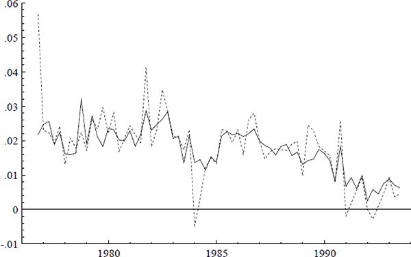
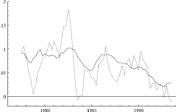
Figure 1 plots the quarterly inflation rates for underlying and headline CPI, denoted Δp and Δph.[3] The most noticeable differences between the two series are in 1976 and 1984, when large changes in the cost of health services occurred. Figures 2 and 3 plot the log of the CPI and its annual growth rate respectively.
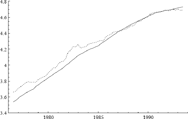
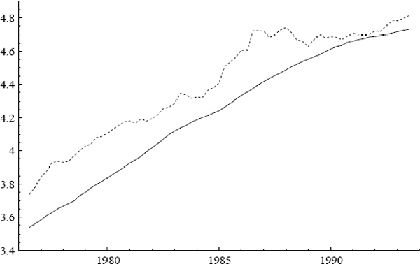
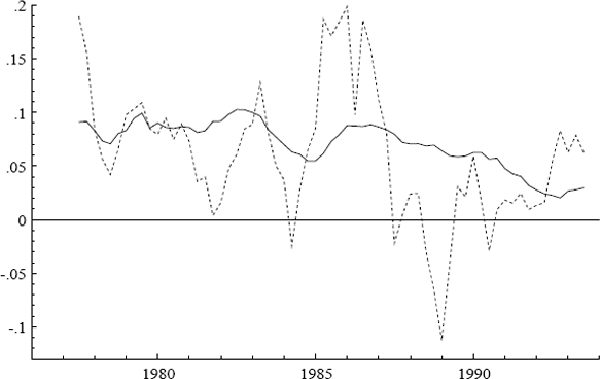
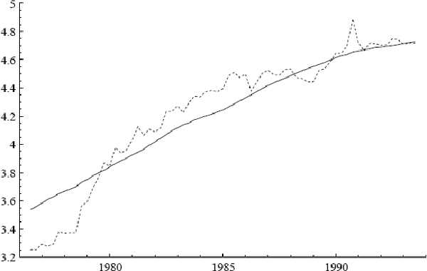
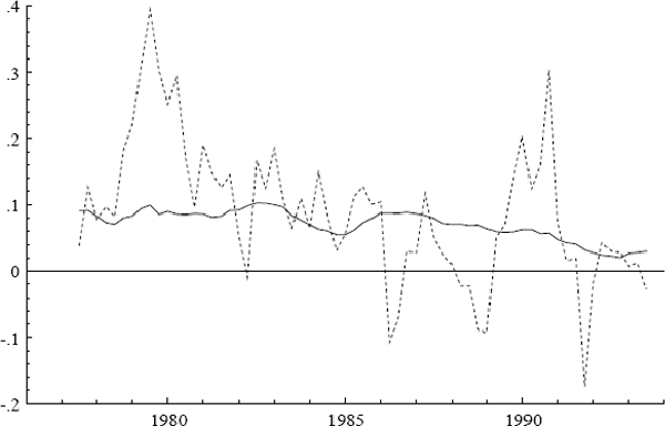
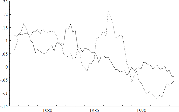
Three additional series are of interest: ULC, IP, and PET. Figures 2–7 plot the logs of these indices and their annual growth rates, contrasting them with the corresponding transformations of the CPI. Over the sample as a whole, unit labour costs and import prices fall relative to the CPI, whereas petrol prices rise relative to the CPI. To make these trends more apparent, Figure 8 plots real unit labour costs and real import prices, and Figure 9 plots real petrol prices. In Figure 8, the two series tend to move in opposite directions by roughly the same magnitude, while having similar downward trends of approximately 1% per annum. Both features are captured more formally in Sections 4.2, 5.2, and 6.1: the first by the nearly equal coefficients on nominal unit labour costs and import prices in the cointegrating vector, the second by inflation's presence in the dynamic steady-state solution for the CPI.[4] In Figure 9, the time series for real petrol prices reflects the OPEC oil price increase in 1979, the fall in real oil prices in the latter half of the 1980s, and the dramatic but temporary increase in oil prices associated with the Gulf War. Further, the growth rates of these possible determinants for the CPI are all much more volatile than the CPI itself: see Figures 3, 5, and 7. Any mark-up model attempting to explain the CPI would need to explain these dramatic differences in variability.
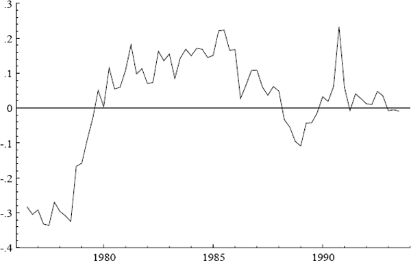
One more series is of interest, private final demand (Y). This series is used to construct a proxy for the output gap, as measured by the residual yres from regressing y on a constant and a trend t. Empirically, regression obtains:
where the estimation sample is 1976(3)–1993(3) and a subscript t denotes time. Equation (5) implies that private final demand is growing at approximately 2.8% per annum on average. The output gap is discussed at greater length in Appendix 3.
The CPI and petrol prices are seasonally unadjusted, whereas unit labour costs, import prices, and private final demand are seasonally adjusted. While such “mixing” of data in the empirical analysis is unfortunate, the alternatives are limited, since the seasonally unadjusted CPI is the variable of interest, and unadjusted data are not available on all of the CPI's potential determinants. See Ericsson, Hendry and Tran (1994) and the papers in Hylleberg (1992) for possible implications of using seasonally adjusted data in economic modelling.
Footnotes
See Reserve Bank of Australia (1994b) for a discussion of related issues and various measurements. [2]
The difference operator Δ is defined as (1 – L), where the lag
operator L shifts a variable one period into the past. Hence, for
xt (a variable x at time t),
Lxt = xt–1 and
so Δxt =
xt–xt–1. More generally,
 .
If i (or j) is undefined, it is taken to be unity.
[3]
To portray clearly the relative movements of ulc – p and ip – p in Figure 8, the mean of ip – p is adjusted when the series are plotted. The means of ulc – p and ip – p are 0.047 and 0.183 respectively, so −0.136 is added to ip – p to bring its mean in line with that of ulc – p. Economically, such adjustment is unimportant: these variables are indices and are in logs. Econometrically, the constant term in a regression induces a similar adjustment. [4]
