RDP 9510: Modelling Inflation in Australia 7. Encompassing and Forecasting
November 1995
- Download the Paper 264KB
Two properties of (17) merit special attention, its ability to account for the results of other models of inflation (encompassing) and its potential usefulness in forecasting. Section 7.1 shows that (17) encompasses an alternate empirical model of inflation due to McTaggart and Hall (1993). Also, at a conceptual level, (17) encompasses several economic models of inflation, while each of those economic models provides only a partial explanation of CPI behaviour in Australia. Section 7.2 examines how (17) might be used for forecasting.
7.1 Encompassing Alternative Models of Inflation
Given the apparent empirical success of (17), it is natural to ask how its performance compares with other models of the Australian CPI. Numerous alternative models have been developed: see for example Fahrer and Myatt (1991), Coelli and Fahrer (1992), the papers in Blundell-Wignall (1992), Johansen (1992b), Knight (1992), and McTaggart and Hall (1993). Several characteristics distinguish (17) from such existing models. First, existing models are typically in differences only, thereby ignoring long-run levels relationships. Johansen (1992b) and Knight (1992) are exceptions in this respect. Second, many of the existing models have apparently significant direct effects of money growth and foreign CPI inflation on Australian CPI inflation. Third, the precise measure of the CPI tends to vary across models. To focus discussion, consider McTaggart and Hall's (1993) model.
McTaggart and Hall (1993) begin with a fourth-order ADL of an adjusted CPI inflation rate (Δpa), an OECD inflation rate (Δp0ECD), the spread between short- and long-term interest rates, and the growth rate of Australian M3 (Δm).[12] From that ADL, they obtained a more parsimonious model:
This model suggests the importance of foreign inflation and domestic monetary expansion as the proximate determinants of Australian inflation, contrasting with the structure in (17). In order to compare these two equations statistically, it is helpful to introduce the concept of encompassing.
Loosely speaking, encompassing is the ability of one model to account for the results of another model. Encompassing is a necessary property for any adequate empirical model: a model's inability to explain the properties of other models indicates the value of information contained in the other models, over and above that in the model being tested. Conversely, the ability of one model to encompass a second model implies that the second is redundant, given the first. Encompassing establishes an ordering across models such that an encompassing model serves as a sufficient statistic for all existing models; cf. Mizon and Richard (1986). Encompassing is particularly important when the alternative models have different economic and policy implications, as they do for (17) and (22).
Numerous test statistics for encompassing have been developed. The ones considered here are due to Cox (1961, 1962) (variance encompassing), Ericsson (1983) (a variant on the Cox statistic), and Sargan (1958) (reduced form encompassing). In addition, the classical F statistic for testing a given model against the smallest comprehensive (nesting) model is included, since that statistic tests parameter encompassing.
Actual implementation of these tests is complicated by different definitions of the CPI, different sample periods for the models, and the lack of seasonal dummies in McTaggart and Hall's equation. To provide as balanced a comparison as possible, each model is tested twice, once using McTaggart and Hall's adjusted CPI and once using underlying CPI. The maximum sample periods available are used in both cases, which are 1977(3)–1992(1) and 1977(3)–1993(3) respectively. While the presence or absence of seasonal dummies is not a formal difficulty for the encompassing tests, seasonal dummies are highly significant if added to McTaggart and Hall's equation. In order to avoid rejecting (22) simply because (17) includes seasonal dummies and (22) does not, the tested version of McTag-gart and Hall's equation includes seasonal dummies. The results appear in Table 3.
| Statistic | Null Hypothesis | ||||||
|---|---|---|---|---|---|---|---|
| Equation (17) | McTaggart and Hall | ||||||
| Dist. | P | Pα | Dist. | P | Pα | ||
| Cox | N(0,1) | −1.82 | −0.98 | N(0,1) | −10.40** | −13.49** | |
| Ericsson | N(0,1) | 1.54 | 0.86 | N(0,1) | 6.00** | 7.38** | |
| Sargan | χ2(4) | 4.91 | 0.85 | χ2(6) | 31.75** | 30.33** | |
| F | F(4, ·) | 1.25 | 0.20 | F(6, ·) | 10.69** | 11.01** | |
 |
0.251% | 0.357% | 0.354% | 0.544% | |||
Notes |
|||||||
From the first two columns of numbers in Table 3, equation (17) appears to encompass McTaggart and Hall's equation. Only the Cox statistic (using P) is at all close to being statistically significant at the nominal 5% level, and the Cox statistic is known to over-reject in finite samples in even static models; see Pesaran (1974) and Ericsson (1986). By contrast, the final two columns in Table 3 show that McTaggart and Hall's equation does not encompass (17), regardless of the statistic used and regardless of the definition of CPI adopted. Put somewhat differently, lagged foreign inflation rates and domestic money growth rates are not important for explaining Australian inflation, conditional on including the growth of petrol prices, the tax dummy, and the lagged output gap and mark-up. Including the tax dummy in McTaggart and Hall's equation does not appreciably alter the results.
From additional similar tests, neither broad money nor short-term interest rates such as the 90-day rate for Bank accepted bills appear to be proximate influences on inflation. That said, monetary policy may and likely does affect inflation. Monetary transmission pathways may include the output gap, the exchange rate, and nominal wage formation inter alia, and through those variables affect inflation. To understand better the monetary transmission mechanism for inflation, a more complete, system analysis would be desirable; but such an analysis is beyond the scope of this paper. For discussion and illustrations of how such an approach would be undertaken, see Hendry and Mizon (1993), Juselius (1993), Doornik and Hendry (1994), and Hendry and Doornik (1994).
The encompassing of (22) by (17) raises an important methodological issue: (22) is a reduced form whereas (17) is “structural”. While comparison of two such models might appear problematic, it is not. The precise meaning of “structural” bears on the explanation itself. First, “structural” sometimes means “conditional”; cf. Boswijk (1995) and Ericsson (1995). Unit labour costs, import prices, and petrol prices are empirically weakly exogenous in (17), so conditioning on their contemporaneous values is valid. In this context, the structural and reduced form aspects of the two models are not at issue. Encompassing simply provides a way of comparing two competing models. Second, and relatedly, the encompassing tests may be viewed as diagnostic checks on the two models. The tests evaluate whether lagged OECD inflation and Australian money growth are important omitted variables in (17), and whether the lagged mark-up and output gap are important omitted variables in (22). None of these variables are precluded a priori from either model, so the nature of an individual model (whether structural or reduced form) does not affect the validity of the encompassing tests. Third, even with empirically valid weak exo-geneity, (17) is in effect a reduced form, with current inflation depending almost exclusively upon lagged information. When contemporaneous unit labour costs and import prices are included in (17), they are numerically and statistically unimportant. Contemporaneous petrol prices, which do appear in (17), are statistically significant but have a very small effect economically. Finally, Hendry and Mizon (1993) show how to calculate encompassing tests between a structural model (their sense of “structural”) and a reduced form, where both are systems. The single-equation encompassing tests above are in the spirit of Hendry and Mizon's tests, noting that super exogeneity appears valid for (17).
At a more conceptual level, (17) encompasses a range of economic models for prices and inflation. Equation (17) embeds a variant of the price-inflation Phillips curve by relating price inflation to the output gap and so to the unemployment rate; cf. Ericsson, Irons and Tryon (1993). When rewritten as (21), (17) also includes both wage-price models (through p – ulc) and long-run purchasing power parity (through p – ip). However, as the empirical model (21) shows, each of these economic theories provides only a partial explanation of price behaviour in Australia. Several economic determinants are necessary to understand the behaviour of the Australian CPI.
Finally, because (17) is empirically constant, broad classes of models may not encompass (17), even in principle. In particular, models of inflation involving rational expectations may not encompass (17); see Hendry (1988), Ericsson and Hendry (1989), Favero and Hendry (1992), and Engle and Hendry (1993). Full testing of such a proposition turns on demonstrating that the equations for ulc, ip, and pet in the VAR are nonconstant. Empirically, the equation for ip appears nonconstant, and possibly those for ulc and pet as well. Again, a more complete, system analysis is the natural framework for testing such propositions but is beyond the scope of this paper.
7.2 Forecasting
Equation (17) is a highly parsimonious model of inflation, making it attractive as a tool for ex ante forecasts and counterfactual simulations. Apart from the current change in petrol prices, CPI inflation in the current quarter is based simply on the levels of the relevant indices and the output gap in the previous quarter. Thus forecasting one step ahead is straightforward. Multi-step ahead forecasts would require forecasts of unit labour costs, import prices, petrol prices, and the output gap, and so would most easily be carried out in a system (rather than a single equation) framework. Ex post forecasts can help assess the constancy of a model, so this subsection considers such forecasts, one step ahead, for the preferred equation.
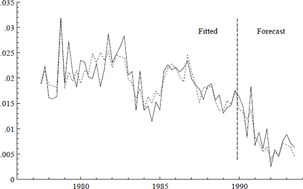
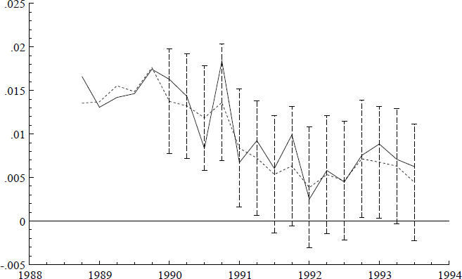
Given recent changes in the Australian economic environment, it is of interest to re-estimate (17) over an initial subsample and use that equation to forecast over the last few years. Figures 17 and 18 plot actual, fitted, and forecast values of inflation, where estimation is through 1989, and realized values of the right-hand side variables are used to construct the forecasts. The forecasts track the recent decline in inflation relatively well. As seen from these forecasts and from the recursive estimates of (17), there is no evidence of a structural break in the inflation process in 1990.


Ex ante forecasts and counterfactual simulations from (17) may be instructive from a policy perspective, but they have several important caveats. First, if only (17) is used, paths for unit labour costs, petrol prices, import prices, and the output gap must be given, precluding feedback from the CPI on to those variables. That is, the CPI is assumed to not Granger-cause the other variables. Second, counterfactual simulations assume robustness of the inflation equation to changes in the processes for unit labour costs, petrol prices, import prices, and the output gap (that is, super exogeneity). Implicitly, that assumes super exogeneity of the exchange rate as well. Third, the forecasts' standard errors are sizable, noting that the equation standard error in (17) is approximately 1% at an annual rate. Typically, multi-step ahead forecast standard errors are larger than their one-step counterparts, with the latter being ±2% (at best) for a 95% confidence region. Finally, actual ex ante multi-step ahead forecasts would require modelling and forecasting the right-hand side variables, and their forecasts are themselves uncertain. Accounting for that uncertainty would almost invariably increase the standard errors of the CPI inflation forecasts. That said, forecasts of the average inflation rate over the next year or two could have a smaller confidence interval than any individual quarter's forecast; see Chong and Hendry (1986) and Campos (1992).
Footnote
McTaggart and Hall's adjusted CPI (Pa) is the headline CPI, net of some (but not all) of the components that were removed from the headline CPI to obtain the underlying CPI. [12]
