RDP 2000-10: Monetary Policy-Making in the Presence of Knightian Uncertainty 4. Knightian Uncertainty and Expected Utility Theory

In cases where there is a single probability distribution over future events, decisions can be made by choosing the action with the maximum expected utility. Savage (1954) and Anscombe and Aumann (1963) provide an axiomatic foundation for this expected utility representation and therefore justify the use of the maximum expected utility decision rule.

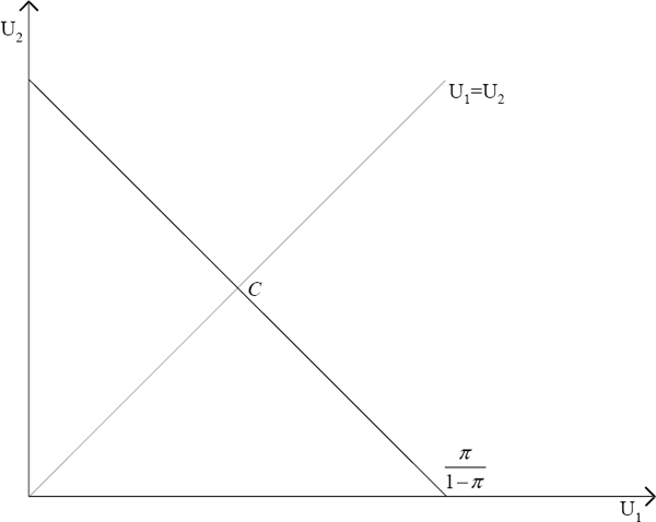
To highlight different approaches to modelling decision-making under Knightian uncertainty, we consider a simple decision problem in which there are two possible states of the world and decision-makers can hold assets that yield utility U₁ in state 1 and U₂ in state 2. Assuming that the probability of state 1 occurring is π, the combinations of U₁ and U₂ that yield the same expected utility will lie on a straight indifference curve with slope , as shown in Figure 1. With gambles along the 45° line, such as C, the decision-maker is certain of getting a particular level of utility regardless of the state of nature that occurs. These gambles will be referred to as constant acts.

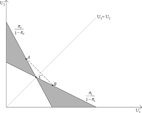
In the case of Knightian uncertainty, the decision-maker applies a range of subjective probability distributions over the possible states of nature. Assuming that the range of probabilities being considered for state 1 is continuous, the lower bound for this probability can be defined as π_L and the upper bound as π_U. The difference between π_U and π_Lcan be thought of as some measure of the degree of Knightian uncertainty facing the decision-maker. In Figure 2, the points that are indifferent to C with respect to a particular probability distribution in this range are represented by the shaded area. Note that the area shaded will become larger the higher the degree of uncertainty.^[1]

Without a unique probability distribution, decisions can no longer be made by maximising expected utility: actions that maximise utility under some probability distributions in the range will not be optimal under others. With this in mind, there have been two main approaches to modelling decision-making under Knightian uncertainty. We present each of these approaches in turn and discuss their implications for the decision rules that should apply. Their implications for monetary policy-making are discussed in Section 5.

4.1 Relaxing the Independence Assumption

The independence assumption has perhaps been the most controversial axiom of expected utility theory since it was formalised by Savage (1954) as the ‘Sure Thing Principle’. The independence axiom states that if A and B are two gambles, and A is preferred to B, that is A B, a mixture of A with a third gamble D will be preferred to a mixture of B and D in the same proportions. That is αA + (1−α)D αB +(1−α)D, where α is strictly between 0 and 1. The indifference curves in Figure 1 are linear if and only if the independence axiom holds.

Gilboa and Schmeidler (1989) argue that the independence axiom will not hold in situations where there is no unique probability distribution, but that a weaker version of independence, which they label constant-independence, will hold. Constant-independence states that if A B, then a mixture of A with a constant act, C, will be preferred to a mixture of B with the constant act C, that is αA +(1−α)C αB +(1−α)C.

The other axiom Gilboa and Schmeidler introduce is uncertainty aversion. Schmeidler (1989) explains that this ‘means that “smoothing” or averaging utility distributions makes the decision-maker better off’. This property arises from the way in which the independence assumption has been relaxed. In situations where there is a single probability distribution, and independence holds, it will be true that if A is indifferent to B, that is A~B, then αA+(1−α)B~αB+(1−α)B=B. Gilboa and Schmeidler show that if the independence assumption is relaxed, it is possible that for A~B, that αA+(1−α)B B for α strictly between 0 and 1 (see below).

Using the weaker definition of independence and introducing uncertainty aversion, Gilboa and Schmeidler (1989) prove that this description of preferences provides a theoretical foundation for Wald's (1950) minimax decision rule. This rule formalises the idea that in situations where there is uncertainty about the probability distribution to apply, decision-makers may choose to minimise the impact of the worst case scenario.^[2] More formally, Gilboa and Schmeidler specify the preference relationship between two gambles, A and B as:

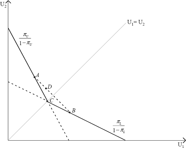
This decision rule allows points that are indifferent to a given constant act, C, to be represented by kinked indifference curves such as the one represented in Figure 3. The transition from Figure 2 to Figure 3 can be explained as follows. Above the 45° line, utility of state 2 is greater than the utility of state 1. The minimum expected utility will be obtained by applying the lowest probability for state 2, that is the highest probability of state 1. Hence, the appropriate slope of the indifference curve above the 45° line is . Using the same argument, the slope of the indifference curve satisfying the minimax rule below the 45° line is . The consequence of the minimax decision rule, therefore, is that Gilboa–Schmeidler preferences are represented by kinked indifference curves, where the kink occurs on the 45° line.

The region above the curve contains points strictly preferred to the points on the indifference curve since each point above the curve gives a higher minimum expected utility. The reverse is true for the area below the curve.

Constant-independence will hold in Figure 3: given that A~B, it is true that

when C is a constant act that lies on the 45° line. To understand how these preferences embody uncertainty aversion, we can see that although the decision-maker is indifferent between A and B, any linear combination of A and B, such as D, is preferred to both A and B. That is, D will yield a higher minimum expected utility than either A or B, despite the fact that A and B will give the decision-maker the same minimum expected utility.

4.2 Relaxation of Completeness

Another approach to describing preferences and decision-making when there is a range of possible probability distributions is to maintain the independence assumption, but relax the completeness assumption. Completeness implies that the decision-maker faced with two gambles will be able to compare them and state a preference relation between them.

Gilboa-Schmeidler preferences are complete because the decision-maker is willing to state a preference between any given alternatives. If, however, a decision-maker thinks that it is important to consider alternatives under the full range of possible probability distributions, it is not possible to reduce the points indifferent to a given constant act to a linear, albeit kinked, indifference curve. Therefore, some points may not be comparable. The possibility of capturing the effects of Knightian uncertainty by dropping the completeness axiom was introduced by Bewley (1986).^[3]

One of the implications of dropping completeness is that it is possible for decision-makers to make a series of decisions that are not consistent with each other. In order to prevent such intransitivity, Bewley introduces the inertia assumption. This assumption states that the decision-maker remains with the status quo unless an alternative that is clearly better under each possible probability distribution is available. This can be thought of as a form of caution: if you are uncertain about whether you will be better off with the alternative, why change your current position?

Bewley preferences imply that faced with two alternatives, X and Y, X will be preferred to Y if and only if E_πU(X)> E_πU(Y) for all π considered. That is to say only when X yields better expected outcomes compared to Y under every distribution will X be preferred to Y.

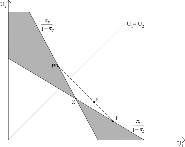
More generally, it can be shown that any point in the shaded region of Figure 4 will not dominate the status quo, Z. For example, a point such as W is better than Z under some probability distributions but worse than Z under others. In this case, the decision-maker does not have any clear preference for either Z or W but because of the inertia assumption, the decision-maker will remain with Z. Point V is clearly better than Z since it gives a higher expected utility under every probability distribution. Should V become available, the decision-maker would choose V over Z. The diagram also indicates that by mixing two gambles, both incomparable to Z, a gamble that is comparable to Z can be produced. So, although the decision-maker will prefer neither W nor Y over Z, the decision-maker will prefer some mixtures of W and Y to Z. The willingness of the decision-maker to make a decision will depend on how much uncertainty exists. The less uncertain the environment, that is, the closer are π_L and π_U, the larger is the set of gambles that are directly comparable to the status quo, and the more likely the decision-maker will be to give up the status quo for an alternative.

Although the inertia assumption gives the decision-maker direction when the decision-maker is faced with incomparable alternatives, it does not provide guidance in situations where there is more than one alternative that strictly dominates the current position. There are a number of possible decision rules that could be used, ranging from rules that recognise the fact that decisions today affect the timing and magnitude of future decisions, to more simple, atheoretical rules such as picking some ‘midpoint’.

Footnotes

For a detailed discussion of aversion to uncertainty, see Epstein (1999). [1]

For monetary policy decision-making, this is similar to minimising the maximum expected loss. [2]

In fact, Bewley asserts that, in his framework, preferences will be complete if and only if there is only one subjective probability distribution. [3]