RDP 2000-10: Monetary Policy-Making in the Presence of Knightian Uncertainty 6. The Optimal Control Problem with Bewley Preferences
December 2000
- Download the Paper 298KB
The difficulty in moving forward is to find a method of incorporating Bewley preferences into an optimal control framework. At a very general level, we want to minimise the policy-maker's loss function subject to the linear constraints that define the dynamics of the economy, the range of expectations the policy-maker has about the distributions of future shocks and the decision rules that are being used. By taking into account all these features, we should obtain internally consistent future paths of interest rates; that is the observed path of interest rates should not be different to the predicted path if no unexpected events occur.
When there is a single probability distribution over future shocks, it is relatively straightforward to obtain the unique, internally consistent path. However, when there is more than one probability distribution, it is much more difficult to obtain this internal consistency, and the uniqueness of the path is not guaranteed. The difficulty can be illustrated through the use of a two-period problem where the Bewley policy-maker must select nominal interest rates for the next two periods, i1 and i2, given their range of subjective expectations.
The policy-maker could begin by choosing an arbitrary value for  .
Given the current state of the economy, the range of subjective expectations and the choice of
 , optimal
control techniques can be applied with each subjective probability distribution in turn, to
generate a range for i1. By applying the decision rule at time t=1,
we can determine the choice of i1, which we denote
  . Taking
this choice of
  and the current state of the economy and
expectations, we can calculate the range of optimal values for i2 . By
applying the decision rule at time t=2, we can determine the choice of
i2 given
  , denoted
  .
If
.
If  , then a
solution has been found. If not, we can iterate on the procedure until a solution is found.
This sketch of the Bewley policy-maker's problem in a two-period setting would be made more concrete by resolving existence and uniqueness issues and proving that if a solution exists, it is internally consistent. It is also clear that it is not straightforward to extend this solution method to the multi-period case as the sequential nature of decision-making is important. The conditions for existence, uniqueness and internal consistency are straightforward in the multi-period case when there is a single subjective probability distribution.
As a first pass at this problem, we assume that the set of probability distributions being considered is convex. In order to establish the range of interest rates that could be optimal, in the next period, we solve the standard optimal policy problem for the probability distributions that form the boundaries of this range. Given convexity, we know that the two period-one interest rates generated from these problems form the boundaries of the feasible range of period-one interest rates, and subsequently the decision rules can be applied. This method ignores the effect of today's decision on the available actions in future periods and implicitly assumes that interest rates after period one will be determined optimally from the probability distribution associated with the chosen period-one interest rate. As such, this algorithm will not be optimal, but might approximate the optimal solution.
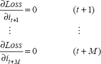
In the general model presented in Section 2, the monetary policy decision-maker chooses interest rates to minimise the loss function in Equation (1). In a finite N period problem, the future path of interest rates can be written as the solution to M=N-(maximum interest rate lag in the output equation) first order conditions:
In the case where there is a single probability distribution, this will yield a unique path of interest rates. In the case where there is a set of probability distributions, it will not. However, it is possible to derive a value for it+1 from a given probability distribution from this range assuming, counterfactually, that future interest rates will be determined as optimal outcomes from this probability distribution.
If the set of probability distributions is convex, the solution to this continuum of problems will yield a range of possible interest rates for it+1. In fact, given convexity, it is possible to find the range by solving for the upper and lower bounds. Once a range for it+1 has been determined, the relevant decision rules can be applied to choose the specific interest rate from the range.
6.1 A Simulation of Monetary Policy in a Simple Model
The model used for the simulations is based on the small closed-economy model used by Ball (1997) and Svensson (1997). The model consists of an equation relating the output gap to its own past behaviour and past real interest rates, and a second equation relating inflation to its history and the past behaviour of the output gap, both estimated over the sample 1985:Q1–2000:Q2.
The output gap used in the model is estimated by fitting a linear trend through real non-farm output from 1980:Q1–2000:Q2. By construction, this output gap will be zero, on average, over the sample period. However, since inflation fell significantly over the sample period, we know that the output gap has been negative on average. Using the methodology outlined in Beechey et al (2000), we reduce the level of the output gap by 3 per cent over the entire sample period. The real interest rate in the output gap equation is calculated as the nominal interest rate, less year-ended inflation. A neutral real cash rate of 3.5 per cent in the model is accepted by the data and imposed. The estimated equation used for the simulations suggests that an increase in the ex post real interest rate of 1 per cent reduces the level of the output gap by 0.12 per cent one year later. The estimation results are presented below (the output gap is measured in per cent), with standard errors in parentheses.
| S.E Regression = 0.65 | Adjusted R-squared = 0.92 |
| DW = 1.88 | Jarque-Bera = 0.40 (P = 0.82) |
The inflation equation is estimated using four-quarter-ended inflation as measured by the Treasury underlying CPI.[4] The most significant difference between the equation estimated for these simulations and the Ball-Svensson model is that it includes changes in, rather than the level of, the output gap. These ‘speed’ terms generate a better fit to the data. The hypothesis that the sum of the coefficients on lagged inflation terms sum to one is accepted and imposed on the equation. The lag structure of the ‘speed’ terms suggests that it takes between a year and eighteen months for changes in the output gap to affect inflation.
| S.E Regression = 0.3 | Adjusted R-squared = 0.99 |
| DW = 1.79 | Jarque-Bera = 3.60 (P = 0.17) |
A number of simulations are presented in this paper. In each simulation, a weight of one has been placed on the inflation objective, measured as squared deviations of year-ended inflation from target, and one-half on the square of the output gap. We have assumed that the target for inflation is 2.5 per cent per annum. As there was no inflation target in place in Australia until 1993, this is when we begin our simulations. A discount factor of one was used in the objective function and in each period, the policy-maker calculates an optimal interest rate path 160 quarters into the future.
The empirical residuals obtained from estimating each of the equations are used as stochastic shocks to the model in chronological order so that the simulated interest rate paths can be compared to the path of the cash rate we actually observe in history. In the simulations, we assume that the policy-maker chooses the nominal interest rate at the beginning of the period, and observes the output gap and inflation at the end of the period. At this time, the policy-maker ‘re-optimises’ to select the nominal cash rate for the following period, assuming the estimated equations are structural. The simulated interest rate paths we obtain are not conditional on the history of actual cash rates observed. In this sense, each of our simulations is dynamic.
As discussed in Section 2, Orphanides (1998) has demonstrated the importance uncertainty about output gap levels and inflation, and consequently the neutral real cash rate, has had on monetary policy decisions in the US. This type of Knightian uncertainty can be translated from uncertainty about variables in the model, into uncertainty about the means of the error distributions and we assume that the policy-maker considers a bounded range of means.
The first simulation is a standard optimal policy exercise that assumes the neutral real interest rate and the state of the economy are known precisely. The second simulation assumes that the policy-maker recognises that their knowledge regarding the neutral real cash rate and the state of the economy is imprecise.
Although we impose the restriction that the neutral real cash rate is equal to 3.5 per cent, the uncertainty that we allow for in the output equation is equivalent to the policy-maker believing the neutral real cash rate could be as low as 3 per cent or as high as 4 per cent. For the inflation equation, we have allowed the means of the shocks to be within one standard deviation either side of zero to incorporate the uncertainties regarding the measurement of inflation and the output gap. The ranges we have selected are somewhat arbitrary and, of course, the ranges could be made wider, smaller, or asymmetric. We also assume for this simulation that the policy-maker chooses the midpoint of the optimal range of interest rates when the inertia assumption cannot be applied.
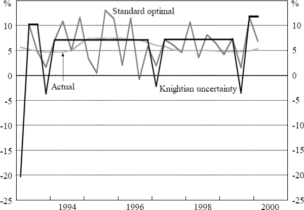
The results of these two simulations are presented in Figure 6. Regardless of whether Knightian uncertainty is included or not, the cash rate paths we obtain from our simulations are quite volatile relative to the path of actual cash rates. Nevertheless, when Knightian uncertainty is allowed for, we obtain extended periods of time where the cash rate remains constant although there are some immediate policy reversals.[5]

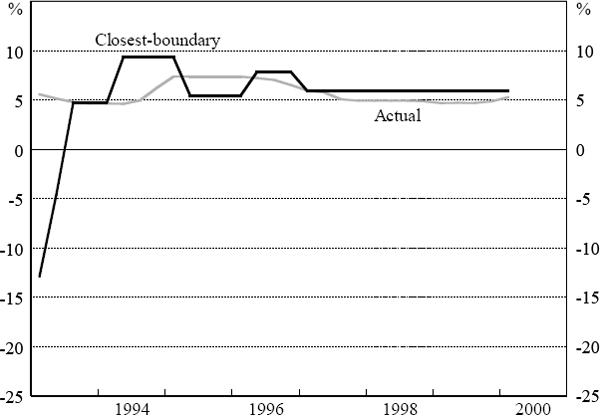
As a point of comparison, we also show, in Figure 7, what the simulated interest rate path would be if we allowed for Knightian uncertainty, but changed interest rates to the nearest boundary of the optimal range, rather than the midpoint, when the inertia assumption does not apply. This rule, that minimises movements in the interest rates, can be argued to be more consistent with the intuitive justification for the inertia assumption in the monetary policy context. This rule also generates an interest rate path with extended periods of no change and no immediate reversals.

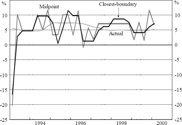
Figure 8 demonstrates the effect of ‘halving’ the degree of uncertainty – that is, halving the range of possible means for the error distribution. In general, less uncertainty implies more changes in interest rates. In the case of the midpoint rule, this means shorter periods of inaction with more frequent, but smaller, policy reversals. In the case of the closest-boundary rule, there are also fewer periods of no change when uncertainty decreases and the length of time between reversals shortens. In practical situations, the degree of uncertainty is likely to change over time. To the extent that points of inflection in the business cycle are periods of relatively high uncertainty, these results can help to explain why interest rates are more stable around turning points.


