RDP 2001-05: Understanding OECD Output Correlations Appendix B: Data
September 2001
- Download the Paper 227KB
We consider 17 OECD countries; these and their associated two-digit ISO codes are listed in Table B1. These countries are selected on the basis of data availability across all of the various bilateral variables we consider.
Output
| Country | ISO code | Quarterly real GDP |
|---|---|---|
| Australia | AU | ABS National Accounts Cat No 5206.0, Table 5 |
| Austria | AT | OEOCGVOLG |
| Canada | CA | CNGDP…D; CNI99BVRG |
| Denmark | DK | DKOCGVOLG |
| Finland | FI | FNI99BVPH |
| France | FR | FRGDP…D; FROCGVOLG |
| Germany | DE | WGGDP…D |
| Italy | IT | ITGDP…D; ITI99BVRG |
| Japan | JP | JPGDP…D; SNA68 |
| Netherlands | NL | NLGDO…D; NLOCGVOLG |
| New Zealand | NZ | NZGDP…D; RBNZ |
| Norway | NO | NWI99BVPH |
| Spain | ES | ESGDP…D; ESOCGVOLG |
| Sweden | SE | SDI99BVPH |
| Switzerland | CH | SWOCGVOLG |
| United Kingdom | GB | UKABMI |
| United States | US | USGDP…D |
Notes: Unless otherwise indicated, codes are for Datastream. Where two sources of data are indicated it is because we do not have an historical series over the 1960–2000 period; series from the two sources are spliced. Some series are not available seasonally adjusted for a substantial portion of the sample; for these series, we use a simple moving average filter as described in Davidson and MacKinnon (1993). |
||
We use quarterly real GDP data to construct four-quarter-ended growth rates (constructed as log fourth differences). The sources for the quarterly GDP data are given in Table B1. To calculate the correlations for the various samples discussed in the text, it is necessary in some instances to take account of the fact that we do not have data for all quarters of the sample. This arises because of limited data, particularly for the earlier years, and also because we use a moving average filter to seasonally adjust some of the series. Where there is missing data, we exclude those observations from the calculation of the bilateral correlations only on a pair wise basis; in other words, for each bilateral correlation, we use the maximum data available.
Bilateral trade in goods and services
The index of bilateral trade intensity we use is the natural logarithm of the following measure:
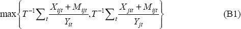
Where Xijt is total nominal exports from country i to country j in period t, Mijt is total nominal imports of country i from country j in period t, and Yit is nominal GDP for country i in period t. All series are measured in USD.
The bilateral trade flows data are from the IMF International Direction of Trade Statistics. For the period 1960–1993, we use the annual data collected by Frankel and Rose (1998) available at <URL:http://www.haas.berkeley.edu/group/eap/>. For the 1993–2000 period, we use the monthly IMF International Direction of Trade Statistics available on Datastream. The monthly data are aggregated to annual data. All series are reported in USD.
Nominal annual GDP is taken from the OECD Economic Outlook, December 2000. The data are converted to USD using year averages of quarterly nominal USD exchange rates for each country. The exchange rate data are from the IMF International Financial Statistics available on Datastream; the codes are reported in Table B2.
| Country |
Nominal annual GDP |
Real annual GDP |
CPI |
Long interest rates |
Short interest rates |
Stock market indices |
Exchange rates |
|---|---|---|---|---|---|---|---|
| Australia | AUOCFGPN | AUOCFGDP | AUOCPCONF | AUI61… | AUOCFIST | AUOCSPRC | AUI..RF. |
| Austria | OEOCFGPN | OEOCFGDP | OEOCPCONF | OEOCLTIR | OEOCFIST | OEI62…F | OEI..RF. |
| Canada | CNOCFGPN | CNOCFGDP | CNOCPCONF | CNOCLNG% | CNOCFIST | CNOCSPRC | CNI..RF. |
| Denmark | DKOCFGPN | DKOCFGDP | DKOCCPNIF | DKOCLTIR | DKOCFIST | DKOCSPRC | DKI..RF. |
| Finland | FNOCFGPN | FNOCFGDP | FNOCPCONF | FNOCLNG% | FNOCFIST | FNOCSPRC | FNI..RF. |
| France | FROCFGPN | FROCFGDP | FROCPCONF | FROCBYG% | FROCFIST | FROCSPRC | FRI..RF. |
| Germany | WGGDP…B | WGGDP…D | WGCP….F | BDOCLNG%R | BDOCFIST | BDOCSPRC | BDI..RF. |
| Italy | ITOCFGPN | ITOCFGDP | ITOCPCONF | ITOCLNG% | ITOCFIST | ITI62…F | ITI..RF. |
| Japan | JPOCFGPN | JPOCFGDP | JPOCPCONF | JPOCLNG% | JPOCFIST | JPOCSPRC | JPI..RF. |
| Netherlands | NLOCFGPN | NLOCFGDP | NLI64…F | NLI61… | NLOCFIST | NLOCSPRC | NLI..RF. |
| New Zealand | NZOCFGPN | NZOCFGDP | NZOCPCONF | NZOCLNG% | NZOCFIST | NZI62…F | NZI..RF. |
| Norway | NWOCFGPN | NWOCFGDP | NWOCPCONF | NWI61… | NWOCFIST | NWI62…F | NWI..RF. |
| Spain | ESOCFGPN | ESOCFGDP | ESOCPCONF | ESI61… | ESOCFIST | ESOCSPRC | ESI..RF. |
| Sweden | SDOCFGPN | SDOCFGDP | SDOCPCONF | SDOCLNGY | SDOCFIST | SDOCSPRC | SDI..RF. |
| Switzerland | SWOCFGPN | SWOCFGDP | SWOCPCONF | SWOCLNG% | SWOCFIST | SWOCSPRC | SWI..RF. |
| United Kingdom | UKOCFGPN | UKOCFGDP | UKOCPCONF | UKOCLNG% | UKOCFIST | UKOCSPRC | UKI..RF. |
| United States | USOCFGPN | USOCFGDP | USOCPCONF | USOCLNG% | USOCFIST | USI62…F | na |
Notes: All series are from Datastream. From 1999, EMU exchange rate data is used for the relevant European countries (code: EMI..RF.) |
|||||||
Bilateral foreign direct investment positions
The index of bilateral trade intensity we use is the natural logarithm of the following measure:
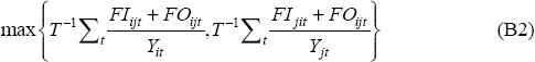
Where FIijt is the inward forward investment position in year t of country i from country j; FOijt is the outward foreign investment position in year t for country i in country j. As before, Yit is nominal GDP for country i in period t and all series are measured in USD. The foreign investment positions are taken from OECD Direct Investment Statistics Yearbook 1999. In most instances, the foreign investment series are reported in local currencies; these are converted to USD using the exchange rate series discussed above.
In theory the numerators of the two indices should be the same, however because they are obtained (by the OECD) from different statistical agencies there can be discrepancies between the figures. By taking the maximum we get a measure of the greatest degree of exposure that two countries might have with each other; it is also consistent with the measure of bilateral trade intensities discussed above.
Real interest rates
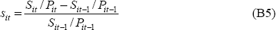
To calculate real interest rates, we use quarterly nominal interest rates and quarterly consumer price indices. From these, we calculate year average interest rates and price levels. Real interest rates are calculated as an ex post measure:

Where iit is the nominal year average interest rate and Pit is the year average consumer price index. For long interest rates, we use long-term government bonds (usually of 10-year maturity). For short interest rates, we use short-term rates (usually of 3-month maturity). For the price level, we use consumer price indices. All series are available on Datastream. The bilateral series used in estimation, for both short and long rates, is the natural logarithm of the standard deviation of the real interest rate spread:

Real equity returns
To calculate real equity returns we use monthly nominal stock market indices and quarterly consumer price indices. From these, we calculate year average levels and use these to calculate real returns over the year:
Where Sit is the value of the stock index in country i in year t and Pit is the consumer price index described above. The stock market indices are monthly and taken, via Datastream, from either the OECD Economic Outlook or IMF International Financial Statistics. The bilateral series used in estimation is the natural logarithm of the standard deviation of the spread on real equity return:

Exchange rate volatility
We use the standard deviation of the quarterly difference, in logarithms, of the nominal bilateral exchange rates. The data is from Datastream; the codes are identified in Table B2.
Bilateral characteristic variables
We use a number of variables in the empirical models, either as instruments or regressors, which are based upon specific economic or geographic characteristics. The variables typically measure whether or not two countries share a particular characteristic. These variables can be grouped as follows: geographic and language, economic size, industry structure, corporate governance, structural economic reform, and the take-up of new technology.
Geographic and language variables
The geographic and language variables we use are bilateral distance, adjacency, and language; these are taken from Frankel and Rose (1998). The adjacency and linguistic dummies are reported in Table B3; the bilateral distance measure is reported in Table B4.
| Upper triangle: adjacency dummy Lower triangle: common language dummy |
|||||||||||||||||
|---|---|---|---|---|---|---|---|---|---|---|---|---|---|---|---|---|---|
| US | GB | AT | DK | FR | DE | IT | NL | NO | SE | CH | CA | JP | FI | ES | AU | NZ | |
| US | 0 | 0 | 0 | 0 | 0 | 0 | 0 | 0 | 0 | 0 | 1 | 0 | 0 | 0 | 0 | 0 | |
| GB | 1 | 0 | 0 | 0 | 0 | 0 | 0 | 0 | 0 | 0 | 0 | 0 | 0 | 0 | 0 | 0 | |
| AT | 0 | 0 | 0 | 0 | 1 | 1 | 0 | 0 | 0 | 1 | 0 | 0 | 0 | 0 | 0 | 0 | |
| DK | 0 | 0 | 0 | 0 | 1 | 0 | 0 | 0 | 1 | 0 | 0 | 0 | 0 | 0 | 0 | 0 | |
| FR | 0 | 0 | 0 | 0 | 1 | 1 | 0 | 0 | 0 | 1 | 0 | 0 | 0 | 1 | 0 | 0 | |
| DE | 0 | 0 | 1 | 0 | 0 | 0 | 1 | 0 | 0 | 1 | 0 | 0 | 0 | 0 | 0 | 0 | |
| IT | 0 | 0 | 0 | 0 | 0 | 0 | 0 | 0 | 0 | 1 | 0 | 0 | 0 | 0 | 0 | 0 | |
| NL | 0 | 0 | 0 | 0 | 0 | 0 | 0 | 0 | 0 | 0 | 0 | 0 | 0 | 0 | 0 | 0 | |
| NO | 0 | 0 | 0 | 0 | 0 | 0 | 0 | 0 | 1 | 0 | 0 | 0 | 1 | 0 | 0 | 0 | |
| SE | 0 | 0 | 0 | 0 | 0 | 0 | 0 | 0 | 0 | 0 | 0 | 0 | 1 | 0 | 0 | 0 | |
| CH | 0 | 0 | 1 | 0 | 1 | 1 | 0 | 0 | 0 | 0 | 0 | 0 | 0 | 0 | 0 | 0 | |
| CA | 1 | 1 | 0 | 0 | 1 | 0 | 0 | 0 | 0 | 0 | 1 | 0 | 0 | 0 | 0 | 0 | |
| JP | 0 | 0 | 0 | 0 | 0 | 0 | 0 | 0 | 0 | 0 | 0 | 0 | 0 | 0 | 0 | 0 | |
| FI | 0 | 0 | 0 | 0 | 0 | 0 | 0 | 0 | 0 | 0 | 0 | 0 | 0 | 0 | 0 | 0 | |
| ES | 0 | 0 | 0 | 0 | 0 | 0 | 0 | 0 | 0 | 0 | 0 | 0 | 0 | 0 | 0 | 0 | |
| AU | 1 | 1 | 0 | 0 | 0 | 0 | 0 | 0 | 0 | 0 | 0 | 1 | 0 | 0 | 0 | 0 | |
| NZ | 1 | 1 | 0 | 0 | 0 | 0 | 0 | 0 | 0 | 0 | 0 | 1 | 0 | 0 | 0 | 1 | |
Source: Frankel and Rose (1998) |
|||||||||||||||||
| US | GB | AT | DK | FR | DE | IT | NL | NO | SE | CH | CA | JP | FI | ES | AU | NZ | |
|---|---|---|---|---|---|---|---|---|---|---|---|---|---|---|---|---|---|
| US | |||||||||||||||||
| GB | 6,360 | ||||||||||||||||
| AT | 7,548 | 1,236 | |||||||||||||||
| DK | 6,847 | 9,57 | 870 | ||||||||||||||
| FR | 6,655 | 341 | 1,035 | 1,028 | |||||||||||||
| DE | 6,839 | 511 | 727 | 659 | 400 | ||||||||||||
| IT | 7,747 | 1,434 | 765 | 1,532 | 1,108 | 1,066 | |||||||||||
| NL | 6,616 | 358 | 935 | 622 | 428 | 235 | 1,295 | ||||||||||
| NO | 6,505 | 1,155 | 1,354 | 485 | 1,343 | 1,048 | 2,009 | 916 | |||||||||
| SE | 6,885 | 1,433 | 1,244 | 523 | 1,544 | 1,182 | 1,978 | 1,127 | 416 | ||||||||
| CH | 7,057 | 748 | 802 | 1,145 | 414 | 509 | 696 | 690 | 1,556 | 1,661 | |||||||
| CA | 1,037 | 5,368 | 6,574 | 5,913 | 5,653 | 5,857 | 6,735 | 5,639 | 5,604 | 5,999 | 6,049 | ||||||
| JP | 10,142 | 9,570 | 9,140 | 8,700 | 9,723 | 9,356 | 9,867 | 9,300 | 8,414 | 8,179 | 9,803 | 10,327 | |||||
| FI | 7,134 | 1,824 | 1,442 | 885 | 1,911 | 1,532 | 2,204 | 1,505 | 789 | 399 | 1,982 | 6,279 | 7,827 | ||||
| ES | 6,733 | 1,265 | 1,810 | 075 | 1,055 | 1,421 | 1,363 | 1,483 | 2,392 | 2,596 | 1,025 | 5,698 | 10,775 | 2,953 | |||
| AU | 14,891 | 17,010 | 15,992 | 16,056 | 16,978 | 16,585 | 16,338 | 16,659 | 15,965 | 15,613 | 16,788 | 15,880 | 7,835 | 15,214 | 17,700 | ||
| NZ | 13,463 | 18,834 | 18,171 | 17,977 | 19,005 | 18,620 | 18,562 | 18,585 | 17,689 | 17,461 | 18,970 | 14,498 | 9,285 | 17,094 | 19,871 | 2,229 | |
|
Note: Distance is between the business centres of the relevant countries measured in kilometres. Source: Frankel and Rose (1998) |
|||||||||||||||||
Economic size
To measure economic size, we use median nominal annual GDP measured in USD for the period 1980–2000. These are constructed from the nominal GDP series identified in Table B2 and converted to USD using the exchange rate series identified in Table B2. For any two countries, we use the natural logarithm of the product of the median GDP measures for both countries as our bilateral index.
Industry structure
This is a measure of the difference between the industry structures of two economies and is based on Imbs (2000); it follows from previous work by Krugman (1991). The index is constructed as follows:
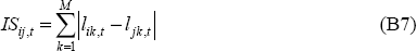
The variable lik,t denotes employment in sector k as a share of total employment in country i. M is the number of sectors and t is the period for which the index is computed. For the empirical work in this paper, we use 1989 data disaggregated to the one digit sector level, which corresponds to the middle of the 1980–2000 sample. The data is from the OECD Labour Force Statistics, various issues.
Corporate governance
We use three variables related to corporate governance taken from La Porta et al (1998). These are country of legal origin, accounting standards and firm ownership concentration. The first identifies the origin of the legal system used by a particularly country; there are four possible groups: English, French, German and Scandinavian. Accounting standards rates each country's accounting standards on a scale of 0–100, with high values indicating good quality accounting standards. Firm ownership measures the concentration of ownership of the top ten non-financial firms for each country. These variables are reported in Table B5.
| Country |
Country of legal origin |
Accounting standards |
Firm ownership |
Structural economic reform |
|---|---|---|---|---|
| United States | English | 71 | 0.12 | 6.50 |
| United Kingdom | English | 78 | 0.15 | 5.81 |
| Austria | German | 54 | 0.51 | 4.50 |
| Denmark | Scandinavian | 62 | 0.40 | 4.81 |
| France | French | 69 | 0.24 | 4.69 |
| Germany | German | 62 | 0.50 | 4.69 |
| Italy | French | 62 | 0.60 | 4.25 |
| Netherlands | French | 64 | 0.31 | 5.00 |
| Norway | Scandinavian | 74 | 0.31 | 4.69 |
| Sweden | Scandinavian | 83 | 0.28 | 5.31 |
| Switzerland | German | 68 | 0.48 | 5.19 |
| Canada | English | 74 | 0.24 | 5.88 |
| Japan | German | 65 | 0.13 | 4.81 |
| Finland | Scandinavian | 77 | 0.34 | 5.13 |
| Spain | French | 64 | 0.50 | 4.50 |
| Australia | English | 75 | 0.28 | 5.38 |
| New Zealand | English | 70 | 0.51 | 5.88 |
Notes: Country of legal origin, accounting standards and firm
ownership are taken from La Porta et al (1998). |
||||
For country of legal origin, we construct a dummy variable that is 1 if a country pair shares a common country of legal origin and 0 otherwise. There are 28 such pairs. We also construct dummy variables specific to each possible origin. For accounting standards, we use as an index the natural logarithm of the product of the two countries accounting standards. We use a similar bilateral index for firm ownership concentration.
Structural economic reform
The structural economic reform bilateral index is constructed from an index prepared by Lehmann Brothers and reported in The Economist (2001). On the basis of a large number of indicators, it rates countries on a scale of 0 to 10 on their structural economic policies (0, worst; 10, best). The measure of structural economic reform for each country is reported in Table B5. The bilateral index is constructed as the natural logarithm of the product of the measures for each country.
Technology adoption
This measures the speed with which a country adopts new technology. We use data on the following three new technologies: mobile phones – number per 1,000 people in 1995; personal computers – number per 1,000 people in 1995 and Internet hosts – number per 10,000 people in 1996. Data on these variables are taken from the World Bank Social Indicators. Countries are ranked according to their adoption of each of the new technologies: those in the top third receive a score of 3, those in the middle third a score of 2 and those in the lowest third a score of 1. The scores are then added across the three technologies to give a total score out of 9. These are reported in Table B6.
| Country | Mobile phones Per 1,000 pop 1995 | Score | Personal computers Per 1,000 pop 1995 |
Score | Internet hosts Per 10,000 pop 1996 | Score | Total score |
|---|---|---|---|---|---|---|---|
| United States | 128.40 | 3 | 328.00 | 3 | 313.16 | 3 | 9 |
| United Kingdom | 98.00 | 2 | 186.20 | 2 | 99.01 | 2 | 6 |
| Austria | 47.60 | 1 | 124.20 | 1 | 88.27 | 2 | 4 |
| Denmark | 157.30 | 3 | 270.50 | 3 | 147.20 | 2 | 8 |
| France | 23.80 | 1 | 134.30 | 1 | 32.69 | 1 | 3 |
| Germany | 42.80 | 1 | 164.90 | 2 | 66.96 | 1 | 4 |
| Italy | 67.40 | 2 | 83.70 | 1 | 19.97 | 1 | 4 |
| Netherlands | 33.20 | 1 | 200.50 | 2 | 138.88 | 2 | 5 |
| Norway | 224.40 | 3 | 273.00 | 3 | 277.46 | 3 | 9 |
| Sweden | 229.40 | 3 | 192.50 | 2 | 211.02 | 3 | 8 |
| Switzerland | 63.50 | 2 | 348.00 | 3 | 145.87 | 2 | 7 |
| Canada | 86.50 | 2 | 192.50 | 2 | 143.33 | 2 | 6 |
| Japan | 81.50 | 2 | 152.50 | 1 | 39.65 | 1 | 4 |
| Finland | 199.20 | 3 | 182.10 | 2 | 542.69 | 3 | 8 |
| Spain | 24.10 | 1 | 81.60 | 1 | 15.93 | 1 | 3 |
| Australia | 127.70 | 3 | 275.80 | 3 | 220.15 | 3 | 9 |
| New Zealand | 108.00 | 2 | 222.70 | 3 | 216.81 | 3 | 8 |
|
Notes: The data are from the World Bank Social Indicators. For each category, ranking is structured as: top 6 = 3; middle 6 = 2; bottom 5 = 1. |
|||||||
An index of difference in speed of adoption is then constructed by taking the absolute difference between the scores of two economies divided by nine. This index then describes how similar two countries are in their adoption of technology.