RDP 2004-09: Co-Movement of Australian State Business Cycles Appendix B: Further Unobserved Components Model Results
October 2004
- Download the Paper 739KB
| State | Trend parameter, δh | Common cycle response parameter, γh | |
|---|---|---|---|
| 1985:Q4–1994:Q4 | 1995:Q1–2003:Q2 | ||
| NSW | 1.86 | 1.35 | 0.51 |
| Vic | 1.22 | 1.12 | 0.59 |
| Q1d | 3.40 | 2.03 | 0.48 |
| WA | 2.69 | 1.66 | 0.54 |
| SA | 0.84 | 0.72 | 0.40 |
| Tas | 0.77 | 0.30 | 0.65 |
| National average | 1.92 | 1.38 | 0.52 |
| Notes: Trend parameter estimates can be interpreted as average annualised percentage growth rates. The ‘national average’ figures are calculated as the average of the state figures, weighted by their share of total hours worked. | |||
| National cycle coefficient, ρ | 0.94 |
|---|---|
National cycle error variance,  |
6.4×10⁻⁵ |
| State | Idiosyncratic cycle response coefficient, θi (for hours worked) |
| NSW | 0.61 |
| Vic | 0.43 |
| Q1d | 0.54 |
| WA | 0.18 |
| SA | 0.25 |
| Tas | 0.21 |
|
Notes: Sample is 1985:Q3–2003:Q2, yielding 71 observations. Idiosyncratic response coefficients for SFD are constrained to equal 1. |
|
| State | NSW | Vic | Q1d | WA | SA | Tas |
|---|---|---|---|---|---|---|
| NSW | 0.83 | −0.08 | −0.10 | −0.07 | −0.07 | −0.11 |
| Vic | 0.20 | 0.58 | −0.11 | −0.02 | −0.35 | 0.05 |
| Q1d | 0.69 | 0.41 | 0.95 | 0.65 | 0.59 | 0.45 |
| WA | −0.63 | −0.53 | −0.52 | 0.46 | −0.61 | −0.14 |
| SA | −0.10 | −0.08 | −0.11 | −0.25 | 0.56 | 0.00 |
| Tas | −0.34 | 0.14 | 0.27 | −0.28 | 0.32 | 0.37 |
| State | Cumulative effect after eight quarters of a shock to: | ||||||
|---|---|---|---|---|---|---|---|
| NSW | Vic | Q1d | WA | SA | Tas | National | |
| NSW | 2.7 | −0.6 | −0.7 | −0.4 | −0.7 | −0.8 | 3.0 |
| Vic | 0.5 | 0.8 | −0.4 | 0.1 | −1.2 | −0.2 | 3.5 |
| Q1d | 0.9 | 0.1 | 1.3 | 0.9 | 0.7 | 0.6 | 2.8 |
| WA | −1.6 | −0.5 | −0.3 | 0.4 | −0.5 | −0.2 | 3.2 |
| SA | 0.5 | 0.2 | 0.2 | −0.3 | 0.9 | 0.1 | 2.4 |
| Tas | 0.5 | 0.5 | 0.5 | −0.1 | 0.7 | 0.7 | 3.9 |
|
Notes: The cumulative response is effectively the integral between the shocked level of hours worked and the no-shock counterfactual level from the shock quarter to the eighth quarter following the shock. The shocks to state idiosyncratic cycles are scaled to increase SFD in the shock state by 1 per cent in the first quarter; the shock to the common cycle is similarly scaled and is 1.95 per cent (see notes to Table 5). All shocks last one quarter, but the model dynamics imply a sustained decay path in each case. |
|||||||
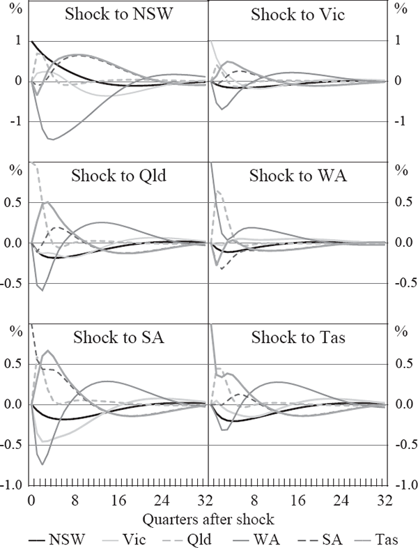
Figure B1: Idiosyncratic Cycle Impulse Response Functions
SFD and hours worked model

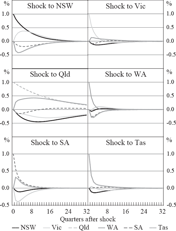
Figure B2: Idiosyncratic Cycle Impulse Response Functions
SFD and hours worked model – suppressing interstate
responses of WA and Qld
