RDP 2004-09: Co-Movement of Australian State Business Cycles 3. Statistical Approaches
October 2004
- Download the Paper 739KB
3.1 The Extent of Co-movement
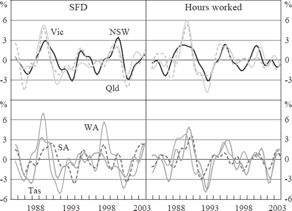
In constructing a measure of ‘the cycle’, one must choose a method of removing high-frequency noise from the data. Our primary method follows the growth cycles literature, whereby trends and volatility are removed from the data using Baxter and King's (1999) band-pass filter.[4] This filter was chosen in preference to others such as the Hodrick-Prescott filter or first-differencing, because it more effectively removes high-frequency information, and has been shown to introduce less distortion than the Hodrick-Prescott filter when a series is autoregressive (Pedersen 2001). Figure 2 shows the resulting cycles. It is clear from this that there is a high degree of synchronicity, particularly among the larger states.[5]

These visual observations can also be confirmed by examining the cross-state correlation of these band-pass filtered variables shown in Table 1. For our sample size, the correlation between two independent random walks will only exceed 0.29 in absolute value in 1 per cent of random draws.[6] All of the correlations exceed this figure, so we can be reasonably confident that SFD and hours worked for all states are contemporaneously correlated at high levels of significance. The degree of synchronicity is greatest amongst the larger states, with average correlations between NSW, Vic and Qld of 0.73 using SFD and 0.70 using hours worked. Whilst correlations are lower among the smaller states (0.49 using SFD and 0.58 using hours worked), they also point to broadly synchronised cycles. Correlations across these two groups average 0.56 using SFD and 0.65 using hours worked.
| State final demand | ||||||
|---|---|---|---|---|---|---|
| NSW | Vic | Q1d | WA | SA | Tas | |
| NSW | 1.00 | |||||
| Vic | 0.68 | 1.00 | ||||
| Q1d | 0.74 | 0.77 | 1.00 | |||
| WA | 0.43 | 0.70 | 0.67 | 1.00 | ||
| SA | 0.64 | 0.45 | 0.50 | 0.43 | 1.00 | |
| Tas | 0.44 | 0.64 | 0.63 | 0.56 | 0.57 | 1.00 |
| Australia | 0.88 | 0.90 | 0.90 | 0.74 | 0.66 | 0.66 |
| Average | 0.58 | 0.65 | 0.66 | 0.56 | 0.52 | 0.57 |
| Hours worked | ||||||
| NSW | Vic | Q1d | WA | SA | Tas | |
| NSW | 1.00 | |||||
| Vic | 0.68 | 1.00 | ||||
| Q1d | 0.65 | 0.77 | 1.00 | |||
| WA | 0.59 | 0.70 | 0.70 | 1.00 | ||
| SA | 0.53 | 0.65 | 0.61 | 0.53 | 1.00 | |
| Tas | 0.73 | 0.68 | 0.64 | 0.58 | 0.62 | 1.00 |
| Australia | 0.87 | 0.92 | 0.88 | 0.79 | 0.71 | 0.78 |
| Average | 0.64 | 0.70 | 0.67 | 0.62 | 0.59 | 0.65 |
|
Notes: Average correlations are calculated over state-state correlations, and exclude correlations with Australia. Data for ‘Australia’ are the band-pass filtered sum of all six states' SFD or hours worked. |
||||||
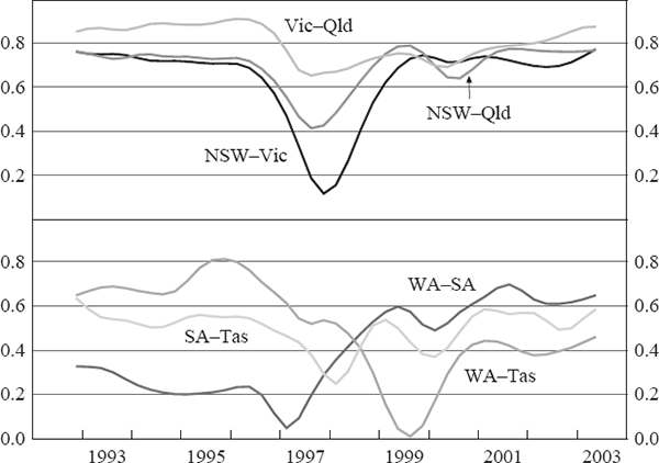
To assess whether the degree of synchronicity has changed substantially over our sample, we computed rolling correlations using a 30-quarter window. The results suggest that there has been no significant change in the degree of co-movement among the larger states, with the exception of the period around 1997–1998 (Figure 3, top panel). The declining correlation of state cycles in that period reflects the staggered entry into, and recovery from, the early 1990s recession across states, and the effect that this has on the rolling correlations as the recession period rolls out of our 7½ year window. The degree of synchronicity among the smaller states has been less stable (Figure 3, bottom panel), with the Western Australian and South Australian cycles increasingly correlated, but the Western Australian and Tasmanian economies increasingly divergent.

Note: Rolling correlations use 30-period windows, plotted relative to the sample end date.
An alternative way to assess co-movement is to consider classical business cycles, which are dated without removing trend growth. Although the literature since Burns and Mitchell's (1946) seminal paper has concentrated more on (detrended) growth cycles, some authors (for example, Harding and Pagan 2002) criticise this approach because it requires imposing a particular structure on the (unknown) trend. As shown by Canova (1998), changes in the trend specification can indeed produce significant differences in the characteristics of the resulting cycles.
A well-known method for dating classical cycles is that set out in Wecker (1979), that two quarterly declines in activity represents a recession, while two successive quarters of growth represents an expansion. On this basis, peaks in activity are defined as periods where {Δyt>0, Δyt+1<0, Δyt+2<0}, while troughs are dated by reversing the inequalities. This algorithm corresponds to a minimum peak-to-peak cycle duration of five quarters, as generally assumed in the literature (Harding and Pagan 2002). It also ensures that an expansion will only be recorded if a series is increasing. However, it does not ensure that an expansion will be recorded if a series is generally increasing, as the series may not record two consecutive quarters of growth.[7] Consequently, for such periods, we supplement this algorithm with the Bry and Boschan (1971) method, now associated with the NBER, to ensure that the absence of two consecutive quarters of growth does not cause a period of generally rising activity to be characterised as an extended recession (nor a decreasing series as an expansion).[8] Applying this technique to Australian data shows that there was a relatively co-ordinated recession between 1989 and 1991. While downturns were observed on other occasions in the sample period in particular states, these were not concurrent across all states.
The degree of similarity between states' classical business cycles can be assessed using the statistical framework provided by Harding and Pagan (2002). They suggest examining the degree of concordance between two states' cycles, using the measure:
where Sjt represents the business cycle phase of state j at time t (1 represents expansion, 0 contraction). This measure ranges between 0 and 1, with 0 representing perfectly counter-cyclical business cycles, and 1 perfectly synchronous cycles. For two cycles described by random walks, the measure will be 0.5 in the limit.
The degree of concordance between each cycle is shown in Table 2. At first glance, these results portray a quite high degree of synchronicity, with most values around 0.7 or above. However, some care must be taken in interpreting these figures. Expansions in each state are highly persistent because trend growth is positive. The expected value for each coefficient is therefore greater than 0.5 – in most cases, somewhat above 0.6.[9]
| NSW | Vic | Q1d | WA | SA | Tas | |
|---|---|---|---|---|---|---|
| NSW | 1.00 | |||||
| Vic | 0.82 | 1.00 | ||||
| Q1d | 0.81 | 0.82 | 1.00 | |||
| WA | 0.81 | 0.77 | 0.76 | 1.00 | ||
| SA | 0.74 | 0.68 | 0.64 | 0.69 | 1.00 | |
| Tas | 0.72 | 0.70 | 0.66 | 0.61 | 0.78 | 1.00 |
| Australia | 0.92 | 0.91 | 0.81 | 0.86 | 0.69 | 0.69 |
| Average | 0.78 | 0.76 | 0.74 | 0.73 | 0.71 | 0.69 |
|
Note: Average concordance is calculated over state-state concordances, excluding the concordance with Australia. |
||||||
Furthermore, it is important to remember the statistical error associated with our estimates, particularly given the small sample size with which we are working. Using a test statistic proposed by McDermott and Scott (2000), we find that 11 of the 21 concordance measures in Table 2 are significant at the 5 per cent level, and 15 at 10 per cent.[10] Tests involving at least one of NSW, Vic and WA tend to be significant, while very few relationships involving SA are significant, even at the 10 per cent level.[11] We take these results to be quite strong evidence in favour of co-movement, given our small sample size.
3.2 Why State Cycles Might Co-move: Preliminary Observations
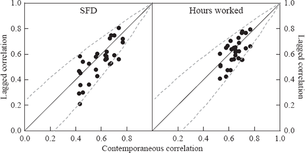
Following the framework described in Section 2, the considerable co-movement documented above could be the result of common shocks, spillovers of idiosyncratic shocks, or a combination of the two. To distinguish between the competing explanations, we use the identification assumption that is standard in the literature, that common shocks affect all states in the same quarter, while spillovers affect states with a lag. Given this assumption, a higher correlation between activity in one state and lagged activity in another (than between activity in these states contemporaneously) would therefore be evidence that spillovers are more important than common shocks. To judge whether this is the case, we plot correlations of SFD in Figure 4, where each dot represents a pair of states. The horizontal axis measures the contemporaneous correlation between these states, and the vertical axis measures the correlation when one state is lagged a quarter. Observations above the 45-degree line represent state pairs where the lagged correlation exceeds the corresponding contemporaneous correlation, suggesting that spillovers are important in explaining co-movement between these states.

Note: Dashed lines are explained in text, and are included only as a rough guide to 95 per cent confidence intervals.
Conducting a formal test of whether each lagged correlation is significantly different from its corresponding contemporaneous correlation is not a straightforward task, since it involves making assumptions about the behaviour of the underlying data. As a rough guide, the dashed lines in Figure 4 depict the 95 per cent confidence bounds which would be obtained if (together with a number of other assumptions) the SFD data for each state pair came from a bivariate normal distribution with no serial correlation. This is clearly not a realistic assumption, because it implies no autocorrelation in state activity, but these confidence intervals do provide a very broad indication that few of the lagged correlations are likely to be significantly greater than the contemporaneous correlations. This suggests that common shocks may be more important in driving co-movement than spillovers. A possible exception to this is WA, whose lagged activity tends to be more highly correlated with contemporaneous activity in other states, indicating that WA's resource-based economy might tend to lead activity in other states. This might occur in several ways. Because of its openness, movements in exchange rates or the terms of trade may affect WA more quickly than other states. In addition, the capital-intensive nature of the mining sector in WA might result in demand-side shocks for WA's resources being transmitted to other states as the need for mining-related capital rises or falls.
Granger causality tests are a second method that can provide guidance on the extent to which spillovers might drive co-movement. A finding that one state Granger-causes another (but not vice versa) would suggest that shocks from that state may indeed spill over to other states. Consequently, we tested for the presence of Granger causality between states, and between each state and the national cycle excluding that state. To account for the presence of unit roots in our series, both SFD and hours worked were first-differenced prior to testing.
Only 4 of the 30 state pairs using SFD, and 9 using hours worked, indicated Granger causality at the 5 per cent level of significance, with no evident pattern in the significant relationships. The higher number of significant relationships using hours worked may reflect that measure's inclusion of the traded sector. However, even taking the results using hours worked as more indicative of state interactions, these results suggest that spillovers play only a small role in driving co-movement, providing support to our earlier findings based on lagged correlations.
We also considered a role for industrial structure in creating cyclical co-movement, given the traditional assumption that it is important. However, comparing Krugman's (1991) industrial dissimilarity index for state pairs with correlations between state cycles, we found little evidence that industrial structure is important, consistent with other research (see, for example, Clark and Shin 2000); our results are presented in Appendix A. Consequently, we have chosen not to further explore industrial structure in our formal examination of the factors accounting for business cycle co-movement.
Footnotes
A band-pass filter is the difference between a low-pass filter (which removes all fluctuations with periodicity less than or equal to some threshold) and a high-pass filter (which removes all fluctuations with periodicity greater than or equal to some other threshold). We choose these thresholds to be 6 and 32 quarters, to match Burns and Mitchell's (1946) definition of a business cycle. [4]
A 6,32 band-pass filter removes the first and last 12 observations. Given our short sample (1985:Q3–2003:Q4 for SFD and 1984:Q4–2003:Q4 for hours worked), we consider this an unacceptable data loss. To correct this, we used trends to extrapolate each series beyond their start and finish point, and allowed the band-pass filter to remove these observations. Consequently, the endpoints of our series are less reliable than their midpoints and should be interpreted with caution. [5]
Our calculations are based on the approximate z-statistic for hypothesis tests
of correlations described in Miller and Miller (1999, p 477). For a test against the
null of zero correlation, the statistic  is approximately
standard normal, where r is the correlation coefficient and n = 71 and
74 is the sample size for SFD and hours worked.
[6]
A series may be increasing, but not record consecutive quarterly growth, if the magnitude of the expansionary quarters outweighs the magnitude of the contractionary quarters. [7]
In such situations, Bry and Boschan's algorithm, which dates peaks in activity as occurring when {yt > yt±k}, with t = 1,2, allows such periods to be classified as expansions. [8]
The expected value is calculated by replacing Sjt and
Skt in Equation (1) with the proportion of time each series spends
in expansion. Denoting this average proportion as  , the expected value will
equal
  (Harding and Pagan 2002). The closer
  and
and
 are to 0.5, the closer the expected value will be to 0.5.
[9]
The test relies on the ratio of the drift of a series (i.e. its trend growth) to its standard error, as well as the sample size. McDermott and Scott (2000) present coefficient weightings for these variables based on Monte Carlo simulations. [10]
South Australia is included in all but two of the relationships that are insignificant at 10 per cent. [11]
