RDP 2011-02: Long-term Interest Rates, Risk Premia and Unconventional Monetary Policy 4. Dynamics

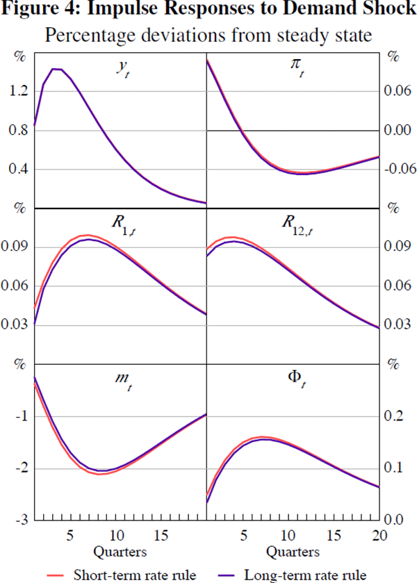
We compute impulse responses using the parameter values of Table B1. Figure 4 shows responses to a demand shock under the Taylor rule and under a long-term interest rate rule using , which at a quarterly frequency corresponds to a 3-year rate. The differences in the responses come from differences in the maturity of the interest rate of the policy rule.

Under both rules, output, inflation, and nominal interest rates rise for the first few periods. Indeed, the responses of all other variables are qualitatively similar and quantitatively close. The long-term interest rate rule gives rise to sensible dynamics. This is also true of the responses to other shocks.

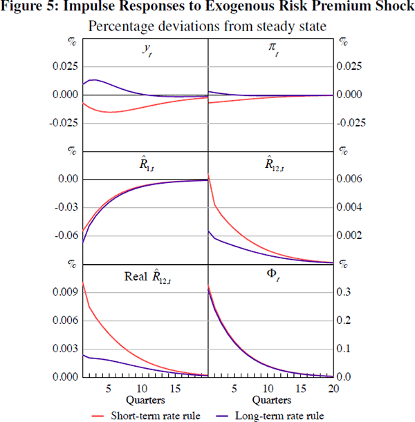
Figure 5 shows responses to an exogenous risk premium shock under both rules. The responses are noticeably different. Under the Taylor rule, output and inflation both decline, whereas under the long-term interest rate rule, output and inflation rise. Because monetary policy sets but Equation (7) holds, the shock to the risk premium is absorbed by a lower sequence of short rates. This lower sequence is expansionary for unrestricted agents who can access short-term borrowing. As a result, output and inflation rise. In the case of the Taylor rule, rises by more, increasing the cost of borrowing for restricted households. As a result, output and inflation fall. In line with Jordan and Peytrignet (2007), financial shocks impact differently on the macroeconomy if policy is set with a longer-term interest rate rule.

If the short-term interest rate were allowed to offset movements in the risk premium, Φ_t , by the inclusion of the risk premium in the policy rule, Equation (5), the responses would be almost identical to those of a central bank that uses a long-term interest rate rule. However, this equivalence, of course, would break down if the zero lower bound were to prevent the short rate from offsetting increases in the risk premium.^[12]

Equation (7) holds regardless of the central bank's choice of policy rule. In particular, Figure 5 suggests that different rules give rise to different yield curve dynamics. To explore the impact of the maturity of the monetary policy instrument, Table 1 shows the standard deviations of and , of the expectation of future short rates, and of the risk premium implied by rules of different maturities. The parameter values of the policy rule are fixed to the values in Table B1, that is, ρ_R = 0.75, ρ_y = 0.09, ρ_π = 0.49 and ρ_µ = 0.35, so differences come only from maturity.^[13] The standard deviations of short and long rates fall as the maturity of the instrument increases. Consistent with this, the standard deviation of the sum of future expected short rates also falls. The volatility of the risk premium under the Taylor rule is about the same than when the instrument is R₁₂, and falls when instruments of longer maturity are used. This mirrors the volatility of money demand across the different policy settings.

Different rules generate different dynamics. So, how do the rules perform? The next section addresses this question.

Footnotes

In practice, in setting monetary policy central banks can take into account variables such as the risk premium. Battellino (2009) notes how the Reserve Bank of Australia has taken into account interest rate spreads, which capture risk premia, in setting interest rates in the recent episode. [12]

The policy shock is set to zero for comparability across the rules. [13]