RDP 2012-08: Estimation and Solution of Models with Expectations and Structural Changes 4. Numerical Examples
December 2012 – ISSN 1320-7229 (Print), ISSN 1448-5109 (Online)
- Download the Paper 1.08MB
4.1 A Credible Disinflation
In this example there is a credible disinflation in the context of the standard New Keynesian model described below in Equations (21)–(27).[6]
In the equations above, xt is the output gap defined as the deviation of output from a socially efficient level of output; πt is the gross rate of inflation, that is ln(pt/pt−1); rt is the log of the gross nominal interest rate; gt is the growth rate of output; ŷt is the percentage deviation from steady state of the log of the stochastically detrended level of output. The log of total factor productivity follows a unit root with a drift, g. Finally, at is a demand shock, et is a cost-push shock and εz,t is the shock to total factor productivity. The ε's are identically and independently distributed shocks.
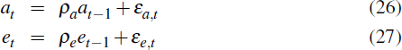
We construct a sample of 200 observations from this system with the following characteristics.
First, the initial structure (model 1) shown in Table 1 governs the system
up to period 159. Second, at the beginning of
period 140, the monetary authority announces a disinflation program
that involves a lower inflation target
(π = 0.0125)
and a more aggressive response to deviations of inflation from this
target (ρr
and ρπ increase).
The response to deviations of growth from trend also increase (ρg
increases). This new policy will be implemented in period 160. Finally, there
are no further structural changes until the end of the sample in period 200.
Agents believe the announcement and revise their expectations accordingly.
In terms of the sample parameters given earlier, T = 200,
Ta = 140 and
 = 160. The parameters of the modified
system are then shown in lower panel of Table 1 while data on the observable
variables, rt, πt
and gt are shown in Figure 3.
= 160. The parameters of the modified
system are then shown in lower panel of Table 1 while data on the observable
variables, rt, πt
and gt are shown in Figure 3.
| Initial structure | |||
|---|---|---|---|
| σr = 0.0017 | σa = 0.0100 | σe = 0.0018 | σz = 0.0040 |
| ρr = 0.7 | ρπ = 0.3 | ρg = 0.1 | ρx = 0.05 |
| β = 0.9975 | ψ = 0.1 | ω = 0.1 | ρa = 0.85 |
| ρe = 0.85 | g = 0.005 | π = 0.05 | r = π + g – lnβ |
| Final structure | |||
| σr = 0.0017 | σa = 0.0100 | σe = 0.0018 | σz = 0.0040 |
 = 1.0 = 1.0 |
 = 0.8 = 0.8 |
 = 0.3 = 0.3 |
ρx = 0.05 |
| β = 0.9975 | ψ = 0.1 | ω = 0.1 | ρa = 0.85 |
| ρe = 0.85 | g = 0.005 | π′ = 0.0125 | r′ = π′ + g – lnβ |
| Announcement and sample size | |||
| T = 200 | Ta = 140 | = 160 |
|
In estimation, rt, πt, and
gt are taken to be observed without noise, that is
V = 0. For our choice of observables, ω is unidentified.
Moreover, in practice it is typically the case that β is not
estimated. For these reasons we set these parameters prior to estimation. The
task is then to estimate the values of the remaining 17 parameters,
 .
.
The results are given in Table 2. The point estimates obtained with the history of observables in Figure 3 correspond to the MLE column in Table 2. The standard error of the maximum likelihood estimators are computed using the theoretical bootstrap with 250 replications. That is, we generate, at the estimated values of the parameters, 250 histories for the observables and estimate the parameters each time.
| Parameter | True value | MLE | Standard error(a) |
|---|---|---|---|
| σr | 0.0017 | 0.0017 | 0.00060 |
| σa | 0.0100 | 0.0106 | 0.00487 |
| σe | 0.0018 | 0.0016 | 0.00220 |
| σz | 0.0040 | 3.0×10⁻⁵ | 0.00331 |
| ρr | 0.70 | 0.7007 | 0.028 |
| ρπ | 0.30 | 0.2994 | 0.033 |
| ρg | 0.10 | 0.1001 | 0.068 |
| ρx | 0.05 | 0.0384 | 0.079 |
| ψ | 0.10 | 0.0739 | 1.749 |
| ρa | 0.85 | 0.8195 | 0.064 |
| ρe | 0.85 | 0.8684 | 0.072 |
| g | 0.0050 | 0.0048 | 0.0002 |
| π | 0.050 | 0.0501 | 0.0047 |
|
|
1.00 | 1.2964 | 0.214 |
|
|
0.80 | 0.8924 | 0.1704 |
|
0.30 | 0.3485 | 0.1038 |
| π′ | 0.0125 | 0.0122 | 0.0005 |
| ℒ | 2,449.62 | 2,507.24 | 38.12 |
|
Note: (a) Based on 25 0 replications |
|||
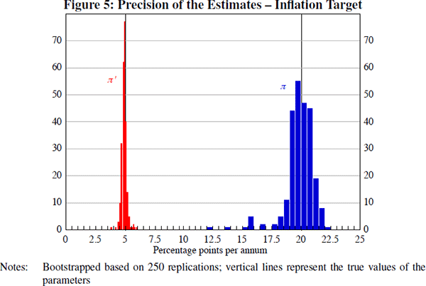
There are three distinct sub-samples in the data. The first 139 observations are constructed using the initial structure (model 1), the last 41 observations are found using the final structure (model 2), and the observations during the transition period – 140 to 159 – involve using both model 1 and model 2 weights when forming expectations. The model parameters that change are those of the monetary policy rule, including the target rate of inflation. As one would expect, because there are more observations generated from the initial structure, the parameters of the initial policy rule are estimated more precisely than those of the final structure. In contrast, because the new policy rule penalises deviations from the new inflation target more strongly, the final inflation target is estimated more precisely. This example illustrates an important point – even though there are relatively fewer observations coming from the final structure, not all of its parameters are estimated less precisely.
These outcomes are illustrated in Figure 4 which shows distributions of the estimators
of the inflation response for both structures, ρπ and
 , and Figure 5 which shows distributions
of the estimators of the inflation targets, π and π′.
, and Figure 5 which shows distributions
of the estimators of the inflation targets, π and π′.
4.2 A Slowdown in Trend Growth
For this example the monetary policy rule, Equation (23), is replaced with

This specification makes a distinction between the inflation target of the central
bank and its estimate of trend growth, πcb and gcb, and those of the private
sector, πand g. For the initial and final structures these
are the same, that is πcb = π and
gcb = g. At Tm = 32 there
is a structural change: g falls to g′ and πcb
increases to
 There is another structural change
at
= 64, when the parameters revert back
to their original values. Unlike the example above, in the period running from
Tm = 32 to
= 64, expectations are (incorrectly)
based on the first model. The reduced-form therefore follows Equation (18).
The parameters of this simulation are summarised in Table 3 along with the
steady state real interest rate for both structures, rr.
There is another structural change
at
= 64, when the parameters revert back
to their original values. Unlike the example above, in the period running from
Tm = 32 to
= 64, expectations are (incorrectly)
based on the first model. The reduced-form therefore follows Equation (18).
The parameters of this simulation are summarised in Table 3 along with the
steady state real interest rate for both structures, rr.
| Initial and final structures | ||
|---|---|---|
| σr = 0.001 | σa = 0.0100 | σe = 0.0030 |
| ρr = 1.0 | ρπ = 0.3 | ρg = 0.2 |
| β = 0.9975 | ψ = 0.1 | ω = 0.1 |
| ρe = 0.85 | g = 0.006 | π = 0.00625 |
| σz = 0.0080 | gcb = 0.006 | πcb = 0.00625 |
| rr = 400(g – lnβ) = 3.4 | ρa = 0.85 | |
| Temporary structure | ||
| σr = 0.001 | σa = 0.0100 | σe = 0.0030 |
| ρr = 1.0 | ρπ = 0.3 | ρg = 0.2 |
| β = 0.9975 | ψ = 0.1 | ω = 0.1 |
| ρe = 0.85 | g′ = 0.0015 | π = 0.00625 |
| σz = 0.0080 | gcb = 0.0060 |
 = 0.02500 = 0.02500 |
| rr′ 400(g′ – lnβ) = 1.6 | ρa = 0.85 | |
| Timing of breaks and sample size | ||
| T = 160 | Tm = 32 |
= 64 |
While the temporary structure is in place trend growth falls. However, the central
bank's view of trend growth does not. At the same time, the central bank
runs looser monetary policy in an attempt to offset weaker growth outcomes.
This is captured by an increase in the central bank's inflation target
to
Agents' beliefs are never updated
and are based on the initial (and final) structure. So in this example,
 , etc and
 , etc. It is therefore unnecessary to
specify Tb
and
, etc. It is therefore unnecessary to
specify Tb
and  . The reduced form therefore
follows Equation (18).
. The reduced form therefore
follows Equation (18).
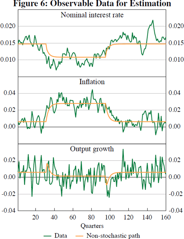
The results are given in Table 4. The point estimates associated with the history of observables shown in Figure 6 correspond to the MLE column in Table 4. The standard error of the maximum likelihood estimator is, as before, computed using the theoretical bootstrap with 250 replications. Figure 6 shows also the non-stochastic path of the simulation which corresponds to the path the economy would have experienced in the presence of structural changes but in the absence of random shocks.
| Parameter | True value | MLE | Standard error(a) |
|---|---|---|---|
| σr | 0.001 | 0.0011 | 0.0002 |
| σa | 0.010 | 0.0097 | 0.0030 |
| σe | 0.003 | 0.0034 | 0.0017 |
| σz | 0.008 | 1.4×10⁻⁵ | 0.0038 |
| ρr | 1.0 | 1.0166 | 0.0702 |
| ρπ | 0.3 | 0.3221 | 0.0569 |
| ρg | 0.2 | 0.2111 | 0.0344 |
| ψ | 0.10 | 0.1022 | 0.5059 |
| ρa | 0.85 | 0.8166 | 0.0647 |
| ρe | 0.85 | 0.8182 | 0.0826 |
| g | 0.0060 | 0.0054 | 0.0005 |
| π | 0.00625 | 0.0069 | 0.0005 |
| g′ | 0.0015 | 1.9×10⁻⁸ | 0.0003 |
|
0.0125 | 0.0254 | 0.0008 |
| ℒ | 2,109.95 | 2,115.63 | 17.82 |
| Note: (a) Based on 250 replications | |||
Footnote
See Ireland (2004) for more details. [6]