Research Discussion Paper – RDP 2016-08 The Slowdown in US Productivity Growth: Breaks and Beliefs
1. Introduction
In many advanced economies, the pace of recovery from the Great Recession has been unexpectedly slow. The United States has performed better than some other economies in this regard. But even so, the level of GDP remains well below what an extrapolation of its pre-recession trend would imply.[1]
While a temporary contraction in economic activity can plausibly be attributed to factors affecting the demand side of an economy, a prolonged slowdown in growth lends itself to a supply-side explanation. Indeed, a growing literature argues that the long-run, or steady-state, rate of total factor productivity (TFP) growth in the United States is lower now than it was in the past (Gordon 2012; Fernald 2014; Reifschneider et al 2015).[2] Visual inspection of Figure 1, which shows the level and growth rate of US TFP over recent decades, appears to support this conjecture.
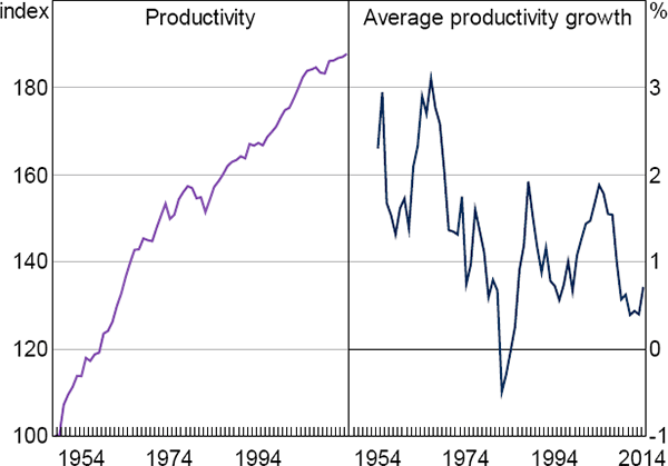
Notes: Left panel shows the log of total factor productivity, normalised to equal 100 in 1948; right panel shows a six-year moving average of annual productivity growth
Sources: Authors' calculations; Bureau of Labor Statistics; Federal Reserve Bank of St. Louis
A downward shift in steady-state US productivity growth matters for several reasons. For US residents, slower productivity growth ultimately means less improvement in living standards. As the United States is responsible for a large part of the world's technological innovation, in as much as US firms operate at the production possibility frontier in many industries, a prolonged slowdown in US productivity growth may limit opportunities for growth in living standards in other countries as well. Slower productivity growth also has implications for monetary policy. In particular, it lowers the neutral real interest rate. For a given inflation target, this implies a lower neutral nominal interest rate. If productivity growth is lower, the zero lower bound on nominal interest rates will bind more frequently.
Yet while much of the recent literature has focused on the possibility of a slowdown in productivity growth, barely a decade ago there was an active debate about whether the arrival of the ‘new economy’, associated with rapid advances in information technology and its diffusion across the economy, marked the start of an era of permanently higher productivity growth (Gordon 2000; Greenspan 2000; Cogley 2005; Kahn and Rich 2007). That such different interpretations of long-run productivity growth can be considered plausible in a short space of time indicates that steady-state productivity growth varies frequently, is difficult to identify in real time, or both.
In light of this, in this paper we explore the timing and size of breaks in US steady-state productivity growth using a business cycle model. A novel feature of our approach is that it allows agents' beliefs about long-run TFP growth to differ from reality. We estimate the model allowing for, but not requiring, breaks in steady-state productivity growth. In the model, shifts in steady-state productivity growth cause predictable changes in economic behaviour. Because agents in the model are forward looking, these changes depend on agents' expectations about productivity growth in the future as well as actual productivity outcomes in the present and the past. In estimation, we infer breaks in steady-state productivity growth, and the beliefs of households and firms about those breaks, from the behaviour of the model's observable variables.
We identify a single break in US productivity growth, most likely occuring in the early 1970s, that roughly halved steady-state growth from 0.6 per cent to 0.3 per cent at a quarterly rate. Relative to the quarter-to-quarter volatility in macroeconomic data, a 0.3 percentage point change in productivity growth might seem inconsequential. But, cumulated over time, even small changes in productivity growth have large consequences. We estimate that per capita consumption and output in the United States would both be around 45 per cent higher today if steady-state productivity growth had not slowed. We also find that the federal funds rate would have been 1 percentage point higher in the mid 2000s and that monetary policy would not have been constrained by the zero lower bound until late 2010.
Our results also indicate that the slowdown in productivity growth was hard to detect in real time. Indeed, the behaviour of households and firms suggests that their beliefs about future productivity growth did not incorporate the slowdown for up to three decades. Because of this delay, the initial responses of output, consumption and investment to the break in productivity growth were smaller than they would have been if agents had observed the break when it occurred. Instead, much of the adjustment occurred after beliefs about steady-state productivity growth shifted down, sometime in the 2000s. This discrepancy between the timing of the break in productivity growth and the time when agents' beliefs about future productivity growth adjusted is a key difference between our results and the recent literature which has identified a downward shift in steady-state productivity growth in the 2000s.
Across a range of specifications we find no evidence of a pick-up in steady-state productivity growth in the 1990s. The productivity growth performance of the United States in this era was extremely strong. But our results indicate that it represented a temporary transition to a higher level of productivity rather than a shift in the steady state of TFP growth. Our results are also robust to a range of other modelling specifications, including allowing for multiple breaks in steady-state growth and for changes in the variance of shocks to productivity growth.
1.1 Relationship to Previous Literature
Our paper builds upon the large body of work that tests for changes in steady-state US productivity growth. One branch of the literature has looked for breaks using univariate statistical models. Early work in this genre tended to find a decline in steady-state productivity growth of around 0.25 percentage points at some point between the late 1960s and mid 1970s (e.g. Dolmas, Raj and Slottje 1999; Benati 2007; Perron and Wada 2009). More recently, with longer samples of data that include the recession of 2007–09, Fernald (2014) and Luo and Startz (2014) identify a larger slowdown in steady-state productivity growth, of 0.4 percentage points, occurring around 2006.
Other authors have adopted a multivariate approach. For instance, Cogley (2005) and Kahn and Rich (2007) use information from consumption and wages, which economic theory predicts will be cointegrated with output, to identify permanent shifts in productivity growth. Both papers conclude that steady-state productivity growth increased in the late 1990s. However, subsequent updates of the Kahn and Rich model suggest that the US economy reverted to a low productivity growth regime in 2005.
Our key contribution to the literature is to explore the timing and size of breaks in US productivity growth through the lens of a business cycle model. Model-based estimates have three advantages over single equation or statistical inferences. First, they use a much broader information set. Changes in productivity growth have implications for many macroeconomic variables. Including these variables in estimation can help to identify the timing and size of breaks in productivity growth. Second, using a structural model allows us to distinguish between shifts in steady-state productivity growth and changes in agents' beliefs about productivity growth. We demonstrate that the response of the economy to changes in steady-state productivity growth depends on whether or not agents' beliefs adjust in real time. Because of this, failing to account for agents' expectations could lead to incorrect inference. Third, by using a structural model, we are able to spell out the implications of slower productivity growth for other macroeconomic variables. In particular, our results shed light on how slower steady-state productivity growth could affect the conduct of monetary policy.
Our work also relates to the growing literature on ‘secular stagnation’, both as a supply-side and demand-side phenomenon.[3] On the supply side, Gordon (2012, 2015) documents a range of demographic, educational, environmental and social factors that he argues will cause US productivity to grow only half as fast in the future as it did on average over the past 150 years. Our results support Gordon's conjecture. In particular, we provide quantitative evidence of a large slowdown in steady-state US productivity growth.
Our results also help to reconcile Gordon's supply-side concept of secular stagnation with that of Summers (2014, 2015), who also raises the prospect of a sustained decline in US economic growth, but identifies demand-side factors as the cause. A key element of Summers' argument is that, since at least the late 1990s, the US economy has failed to achieve strong growth in real economic activity and financial stability simultaneously. This failure could occur in an environment in which agents' expectations about future income growth, which is a key determinant of asset prices, are too optimistic (e.g. Hoffmann, Krause and Laubach 2012). This is precisely the mechanism that we uncover in our paper – steady-state productivity growth fell long before beliefs about future productivity growth adjusted.
The rest of the paper is organised as follows. Section 2 provides details of the theoretical model and illustrates its response to structural breaks in steady-state productivity growth. Section 3 describes the estimation approach. Section 4 presents results and highlights features of the data that influence the estimated timing of breaks in productivity growth. Section 5 discusses some of the implications of our results for the US economy. Section 6 shows the robustness of the estimation results to alternative model specifications. And Section 7 concludes.
2. Model
We work with the model described in Justiniano, Primiceri and Tambalotti (2013). Like other canonical models of the US economy, such as that in Smets and Wouters (2007), this model features a neoclassical core augmented by shocks and frictions that help to explain quarter-to-quarter variation in the data. A desirable feature of the model is that it assumes that TFP growth follows a stochastic trend. A stochastic trend helps the model to account for large and persistent deviations of TFP growth from its steady-state growth rate. This turns out to be important in interpreting the behaviour of the US economy during the 1990s. As the model is standard, we refer readers to Justiniano et al (2013) for a full exposition and Appendix B for the log-linearised equations.
In the model, the growth rate of TFP, zt , follows the stochastic process:
where γ is the steady-state growth rate of TFP, ρz controls the persistence of disturbances to the growth rate of TFP and εz,t represent disturbances to the growth rate of TFP. These disturbances follow an independently and identically distributed process with zero mean and constant variance.
2.1 Modelling Structural Breaks in Productivity Growth
In estimation, we allow for breaks in γ, the steady-state growth rate of TFP. We incorporate these breaks using the methods outlined in Kulish and Pagan (forthcoming). In this section we describe the approach when there is a single break in steady-state TFP growth. It is straightforward to generalise the techniques to cases with multiple breaks.
Let t = 1, 2,…, T represent the periods in the data sample. From period t = 1, 2,…, Tγ− 1 steady-state TFP growth takes some initial value, γi. We work with a linear rational expectations model of n equations that can be written as:
where A0, C0, A1, B0 and D0 are the structural matrices associated with the initial steady-state TFP growth rate, Et is the expectations operator, yt is a n × 1 vector of endogenous variables and εt is an l × 1 vector of exogenous variables. We take the latter to be white noise and to have Iι as their covariance matrix. If a solution to Equation (2) exists and is unique it will be a VAR of the form:
Noting that Etεt + 1 = 0, then if agents know the true structure of the economy it follows that the reduced form coefficients in Equation (3) and structural coefficients in Equation (2) have the relationships:
where  .
.
From t = Tγ, Tγ + 1,…, T, steady-state TFP growth takes some different value, γf. The structural form of the model then becomes:
where the superscript * denotes the matrices corresponding to the new TFP growth rate. If agents'
beliefs about future TFP growth adjust immediately at Tγ then the
solution from this point on is simply  ,
with the reduced form matrices constructed in a similar manner to those in Equations (4)–(6).
As well as changing the dynamics of the system, the shift in steady-state productivity growth
also changes other steady-state values. This means that even in the perfect foresight case, in
which there are no stochastic shocks, a change in steady-state productivity growth will induce
transitional dynamics as the economy moves to its new steady state. The technique described
above accounts for both the change in the model's steady state and the transition.
We also allow for the possibility that it may take time for agents' beliefs about steady-state TFP growth to adjust to the structural change. In this case there is a period of time in which the actual structure of the economy has altered but agents continue to form expectations based upon the original structure. Formally, let Tb > Tγ denote the date at which beliefs adjust. In the intervening period t = Tγ, Tγ + 1,…, Tb − 1, the actual path of the economy continues to obey Equation (7). However, expectations are based on the initial structure of the economy, that is Etyt + 1 = C + Qyt. During this time, the solution of the model is given by:
where
and  and
and  From
t = Tb, Tb + 1,…, T the
solution of the model becomes
  .
.
2.2 Implications of a Change in Steady-state Productivity Growth
A change in γ alters the growth rate of TFP permanently. In contrast, an innovation to εz,t has a temporary (but possibly quite persistent) effect on the growth rate of TFP (although it has a permanent effect on its level). The response of economic variables to temporary and permanent changes in productivity growth differ. This allows us to distinguish between shifts in γ and innovations to εz,t in estimation.
To illustrate this, Figure 2 shows the consequences of a decrease in trend productivity growth for some of the key macroeconomic variables in our model. To construct the figure, we simulate the model for 100 quarters, setting all parameter values except for the one controlling steady-state productivity growth, γ, at the posterior means reported in Justiniano et al (2013). For the first 24 quarters, we set γ equal to 0.50 per cent at a quarterly rate, which is similar to the posterior mean reported in Justiniano et al (2013). In quarter 25, we lower the value of γ by 0.25 percentage points to 0.25. In this example, agents observe the break in steady-state productivity growth when it occurs and adjust their behaviour immediately in response to this change.
In the figure, the lines labelled ‘stochastic’ represent the stochastic simulation of GDP, consumption, investment and real wages growth as well as inflation and interest rates. The lines labelled ‘non-stochastic’ show the non-stochastic path of the variables. This is the path these variables would have followed if the economy experienced no structural shocks but the decrease in steady-state productivity growth still occurred.
Focusing first on the non-stochastic paths, the fall in steady-state productivity growth lowers the growth rate of GDP, consumption and real wages, as expected. The steady-state real interest rate, given by γ/β (where β is the households' intertemporal discount rate), decreases. As the central bank's inflation target remains constant, the steady-state nominal interest rate also falls. It takes a few years for interest rates to reach their steady-state level, however, as the decrease in productivity growth has a modest inflationary impact in the near term.
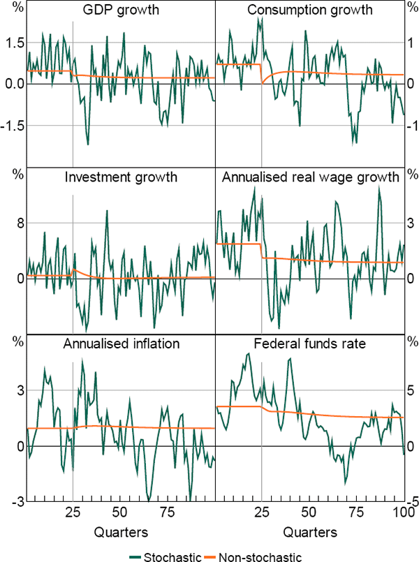
Perhaps the most surprising response is that of investment growth. This increases in the first few quarters after the break, although it ultimately settles at a lower growth rate. The initial increase in investment growth has two causes. First, on the supply side, the desire of households to reduce consumption in response to an unanticipated fall in productivity growth creates additional savings, which firms can use to invest. Second, on the demand side, the price of new capital falls but overshoots its final level. This creates an incentive for firms to invest in the near term while capital is relatively cheap.
In Figure 2 agents observe the break in productivity growth as it happens. In reality, one might think that agents will take some time to realise that steady-state productivity growth has declined. Figure 3 illustrates the non-stochastic paths of the economy when agents' beliefs do not match reality. In this case, we assume that agents' beliefs about steady-state productivity growth do not adjust until quarter 75, that is, around seven years after the break. For comparison, we also graph the non-stochastic paths from Figure 2 (in which agents observe the change in steady-state productivity growth in real time).
The non-stochastic path of the economy in Figure 3 differs in several respects from that of Figure 2. For example, consumption growth falls when the break in productivity growth occurs and then again when agents' beliefs adjust. The first decrease in consumption is smaller, because households initially anticipate that the fall in productivity growth will be temporary. The second decrease is larger because households realise that productivity growth will be slower permanently. Likewise, investment growth increases when beliefs adjust rather than when the break in productivity growth actually occurs.
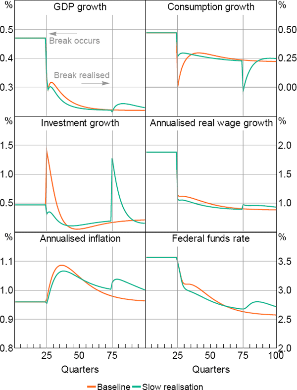
Interest rates initially fall by marginally more when agents' beliefs do not adjust immediately. This reflects the fact that the central bank shares the same information set as other agents in the economy. They perceive the slowdown in economic growth to be cyclical rather than structural and accordingly lower interest rates to combat this.
In contrast, most of the slowdown in real wages growth occurs at the time of the break in productivity growth. In the model, despite the presence of nominal wage rigidities, real wages are less forward looking than consumption. Instead, they are more reflective of recent productivity growth outcomes. Consequently, real wages adjust rapidly to a slowdown in trend productivity growth even if agents perceive the slowdown to be transitory.
The simulations in Figures 2 and 3 show that breaks in productivity growth have implications for many observable macroeconomic variables. In estimation, we use these implications to identify the breaks. The simulations also highlight how the response of the economy depends on agents' beliefs about future productivity growth, pointing to the benefits of structural estimation that can take account of these beliefs.
However, comparing the stochastic and non-stochastic paths in Figure 2 also indicates that the quarter-to-quarter volatility in macroeconomic data could be far greater than the dynamics induced by even a relatively large change in steady-state productivity growth. This raises the question of whether our estimation will be able to identify a break in productivity growth successfully. To address this concern, we estimate the parameters of the model using simulated data. We find that we are able to recover the actual parameters with a high degree of accuracy.[4]
3. Estimation
We estimate the model using Bayesian methods, as is common in the DSGE literature. Our case,
however, is non-standard because we allow for structural change and jointly estimate two sets of
distinct parameters. These are: (i) the structural parameters of the model,  ,
that have continuous support; and (ii) the dates of the structural changes, T =
(Tγ, Tb) that have discrete support. The joint
posterior density of
  and T can be
expressed as:
where  is the data and
  is
an nobs × 1 vector of observable variables.
  is
the likelihood of the model, which we construct using the methods described in Kulish and Pagan
(forthcoming). The priors for the structural parameters and the date breaks are independent, so
that
  . Appendix E describes
the posterior sampler.
3.1 Data
We estimate the model using seven series of US quarterly data: GDP, consumption, investment, inflation, the federal funds rate, hours worked, and nominal wages.[5] GDP, consumption and investment are measured in per capita growth rates, while hours are measured in per capita levels. Appendix A lists the data sources.
Our estimation sample starts in 1964:Q2 and ends in 2014:Q4. From 2008:Q4 to the end of our sample, the federal funds rate was at the zero lower bound. This poses a challenge for our model, which does not allow for nonlinearities in the monetary policy reaction function.
To account for the behaviour of monetary policy at the zero lower bound, from 2008:Q4 to 2014:Q4 we replace the observed federal funds rate with the ‘shadow’ federal funds rate derived by Wu and Xia (2014). This measure quantifies the effective federal funds rate implied by the unconventional monetary policy, such as forward guidance and quantitative easing, undertaken by the Federal Reserve since 2009. For instance, a shadow federal funds rate of −0.5 per cent means that unconventional policy is having the same effect on the US economy as if the Federal Reserve had been able to set the federal funds rate at −0.5 per cent.
An alternative approach would be to incorporate the zero lower bound explicitly in the model and estimation.[6] This approach has two drawbacks. First, it would complicate the estimation of the model, which seems undesirable as the behaviour of the economy at the zero lower bound is not the focus of this paper. Second, after reaching the zero lower bound, the Federal Reserve continued to apply further monetary stimulus to the US economy through unconventional policy actions. Setting the nominal interest rate to zero without taking account of unconventional policy could lead to incorrect inferences about the behaviour and consequences of US monetary policy over recent years.
3.2 Priors
For the parameters of most interest to us, the growth rate of steady-state TFP in the initial regime, γi, and final regime, γf, we impose normal distributions with mean 0.5 and standard deviation 0.2.[7] The mean of this prior distribution is similar to that used in other estimated US DSGE models, but the standard deviation is wider. Note that our prior is agnostic about the direction of the change in US TFP growth. The estimation is free to conclude that steady-state productivity growth has increased, decreased or stayed the same.
For the parameters governing the timing of the break in steady-state productivity growth, Tγ, and beliefs about the break, Tb, we impose uniform priors. We restrict the domain of these parameters to exclude the first and last 5 per cent of observations. This leaves these parameters with an effective domain of 1966:Q3 to 2012:Q2. This window encompasses all of the date breaks typically identified in single equation reduced form estimation.
For the other parameters, we use the same priors as described in Justiniano et al (2013). Most of these priors are reasonably loose and serve mainly to regularise the posterior distribution of the model so that it remains numerically stable and constrain parameter values to be economically sensible.
4. Results
In this section we present results for our preferred model, which features a single break in steady-state productivity growth and allows agents' beliefs about steady-state productivity growth to change at a different date to the actual break. In Section 6, we compare these results to alternative specifications.
The left panel of Figure 4 shows the probability density function (PDF) of the posterior distribution of the timing of the break in steady-state productivity growth. The estimation strongly prefers a break in productivity growth in the early 1970s – the mode of the distribution occurs in 1970:Q4 and the median around one year later. The estimation assigns a small probability to the break occurring in the 2000s. But it has little mass in the 1990s, indicating that the model does not interpret the pick-up in productivity growth at this time as a shift in steady-state productivity growth.[8]
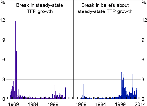
The right panel of Figure 4 shows the PDF of the date at which agents' beliefs about productivity growth changed. The results indicate that the shift in agents' beliefs about steady-state productivity growth occurred well after the actual break. There is substantial mass in the early 2000s, although the mode of the distribution is a bit later, in 2008.
Table 1 documents the estimation results for the remaining parameters of the productivity growth process. The point estimate of the initial steady-state TFP growth rate, γi = 0.59, is slightly higher than reported in other structural models of the US economy (for example, Justiniano et al (2013), which was 0.47, and Smets and Wouters (2007), which was 0.43), although the 90 per cent confidence interval spans these earlier estimates. The estimation points to a large slowdown in steady-state productivity growth after the structural break. In fact, the point estimates suggest that quarterly steady-state productivity growth has almost halved from 0.59 per cent to 0.33 per cent. The estimates of the persistence of the TFP process, ρz, and the standard deviation of shocks to productivity growth, σz, are similar to those reported in Justiniano et al (2013).
| Parameter | Description | Prior | Posterior | |||||
|---|---|---|---|---|---|---|---|---|
| Distribution | Mean | Std error | Mean(a) | Median | 5% | 95% | ||
| Timing of structural breaks | ||||||||
| Tγ | TFP break | U | [1965:Q3–2012:Q1](b) | 1970:Q4 | 1971:Q4 | 1981:Q2 | 1986:Q1 | |
| Tb | Beliefs adjust | U | [1965:Q3–2012:Q1](b) | 2008:Q4 | 2003:Q1 | 1997:Q2 | 2011:Q3 | |
| TFP process | ||||||||
| γi | Initial growth | N | 0.50 | 0.20 | 0.59 | 0.58 | 0.38 | 0.82 |
| γf | Final growth | N | 0.50 | 0.20 | 0.33 | 0.34 | 0.14 | 0.47 |
| ρz | Auto TFP | B | 0.40 | 0.20 | 0.06 | 0.06 | 0.01 | 0.14 |
| 100σz | Std dev TFP | IG | 1.00 | 1.00 | 0.90 | 0.90 | 0.82 | 0.99 |
| Marginal data density: −1,236.7 | ||||||||
|
Notes: U denotes uniform distribution, N denotes normal distribution, B denotes
beta distribution, and IG denotes inverse gamma distribution |
||||||||
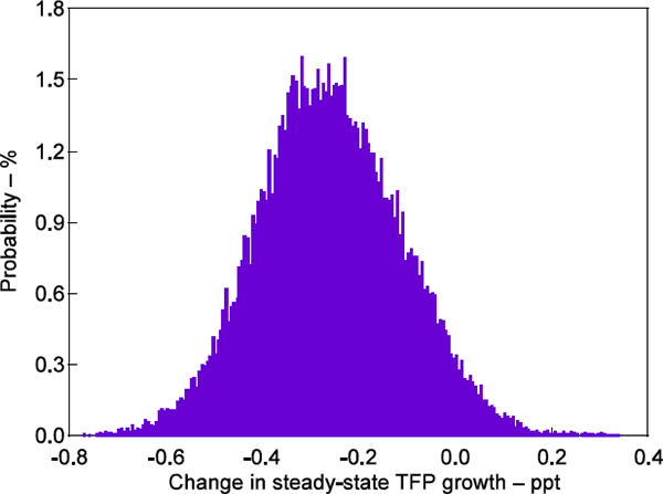
Our finding of a slowdown in steady-state productivity growth is economically meaningful. But is it statistically so? We present two pieces of evidence to suggest that it is. First, Figure 5 shows the posterior distribution of the change in productivity growth between the initial and final steady states. To construct this figure we compute the difference between the final steady-state productivity growth rate and the initial rate (that is, (γf − γi) for each draw from the posterior distribution and plot the histogram of these values. The 90 per cent highest probability interval for this distribution spans −0.49 to −0.01. That is, the estimation finds little evidence that the steady-state productivity growth rate has increased or even stayed the same.
Second, we re-estimated the model without allowing for a structural break in TFP growth (or beliefs about TFP growth). The marginal data density of our baseline model is −1,236.7. The marginal data density of the no-breaks model is −1,238.4. A standard metric for model comparison is twice the log Bayes factor, which in this case is equal to 3.3. Using the criteria of Kass and Raftery (1995), this provides positive evidence in favour of a model that allows for a break in productivity growth.
Appendix C contains estimation results for the other parameters of the model. For the most part, these parameter estimates are very close to those reported in Justiniano et al (2013). That is, while we find strong evidence that there has been a slowdown in the steady-state productivity growth rate, ignoring this slowdown does not appear to change the other estimated properties of the model.[9]
4.1 Why Do We Find the Breaks Where We Do?
In this section we discuss why the estimation identifies break dates where it does. We first highlight features of the data that lead the estimation to identify breaks in the 1970s and 2000s. We then discuss why the data does not identify a break in the 1990s, as some previous research has.
4.1.1 Why do we estimate a break in trend productivity growth in the 1970s?
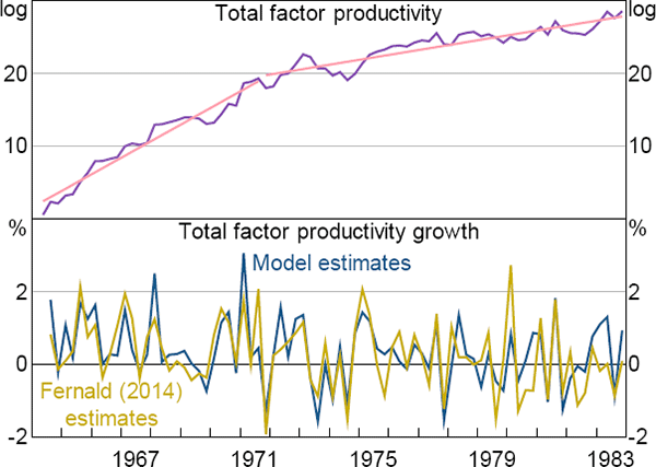
A natural starting point to understand why the estimation identifies a break in steady-state TFP growth in the early 1970s is to look at the behaviour of productivity itself. The top panel of Figure 6 plots the estimated log level of productivity implied by the model (with all parameters set at their posterior median values). The two straight segments plot lines of best fit over the period 1964:Q2 to 1971:Q3 (that is, before the estimated break) and between 1971:Q4 and 1983:Q4 (that is, the 12 years after the estimated break). The slope of the segments clearly declines in the latter period, indicative of a slowdown in average productivity growth.
Sources: Authors' calculations; Fernald (2014)
Of course, productivity cannot be observed directly, and productivity measures may be contaminated by cyclical influences or measurement error. These factors, however, do not appear to be driving the patterns shown in the top panel of Figure 6. To illustrate this, the bottom panel of the figure plots the model's estimated productivity growth series against an alternative series published in Fernald (2014). Fernald constructs a series that accords closely to the theoretical concept of TFP by removing from the official US productivity statistics the effects of variation in the utilisation of capital and labour as well as improvements in the quality of labour. Despite the conceptual differences, our estimates correspond closely to Fernald's series, with a correlation over the sample in the figure of 0.71. Like us, Fernald's series indicates a slowdown in the average pace of productivity growth in the early 1970s.
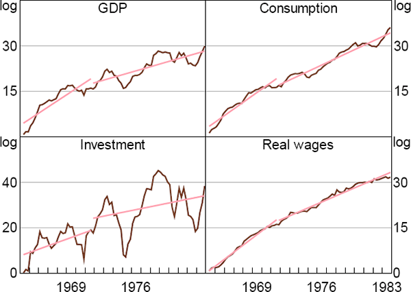
As we emphasised in Section 2, our estimation procedure takes account of the joint behaviour of a range of macroeconomic variables to form inferences about breaks in steady-state productivity growth. Recall from Figure 3 that we should expect a decrease in steady-state productivity growth to lower the growth rates of GDP, consumption, investment and real wages. Figure 7 graphs the evolution of these variables over the period 1964:Q2 to 1983:Q4. As in Figure 6, the straight lines correspond to lines of best fit over the sub-samples 1964:Q2 to 1971:Q3 and 1971:Q4 to 1983:Q4.
Sources: Authors' calculations; Bureau of Economic Analysis; Bureau of Labor Statistics
For all four variables, average growth rates decrease after the estimated break in productivity growth, consistent with the theoretical predictions. The decrease in average consumption growth, however, is modest compared to those of GDP and real wages. This may help to explain why the model assigns little probability to there being a break in agents' beliefs about trend productivity growth at this time.
4.1.2 Why didn't agents perceive the slowdown until the 2000s?
The estimation suggests that beliefs about steady-state productivity growth adjusted in the 2000s, with the periods of greatest probability being 2000–01 and 2008. Both of these date ranges coincided with periods of weak output and consumption growth, consistent with Figure 3. Mechanically, we would expect these patterns to lead the estimation to identify a break in agents' beliefs at these times. But, of course, the recessions of the early 2000s and 2007–09 had a range of causes and one would not attribute them solely to changes in beliefs about future productivity growth. In this section, we show that a downward shift in expectations about future steady-state productivity growth is consistent with the pattern of agents' forecast errors as well as evidence from outside the model.
One reason for scepticism about the three-decade gap that we estimate between the break in steady-state productivity growth and the shift in agents' beliefs is that it seems to imply that households and firms would have made persistent forecast errors for an implausibly long time. It turns out, however, that this is not the case. To illustrate this, Figure 8 plots the cumulative one-step-ahead forecast errors of GDP growth made by agents in the model. The errors account for the fact that, between 1971 and 2003, agents' beliefs about steady-state productivity growth remained at their initial level even though actual steady-state productivity growth had declined.
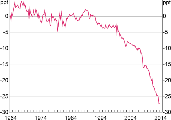
If agents in the model persistently overestimated productivity growth, we would expect to see these cumulative errors become increasingly negative. Such a drift is not apparent until the early 2000s. After that, agents' one-step-ahead forecasts persistently overestimated the actual outcomes of these variables. This pattern of errors is intuitive. As noted above, the 1990s was a time of strong productivity growth in the United States, albeit one that we would argue was driven by temporary factors rather than a permanent shift in steady-state growth. In such an environment, it is natural that agents would have underpredicted future consumption or output growth as often as they would have overpredicted these quantities. Given this pattern of forecast errors, it is understandable that it would take agents many years to revise their beliefs about steady-state productivity growth.
The timing of the shift in agents' beliefs is also consistent with evidence from outside the model. Asset prices are a natural place to look for shifts in beliefs about long-run productivity growth as they should be forward looking and rapidly incorporate new information. Figure 9 plots the NASDAQ and S&P 500 stock market indices over recent decades, with the highlighted areas corresponding to the periods in which our estimation assigns a high probability to beliefs about steady-state productivity growth shifting down. Both periods of high probability coincided with large falls in equity prices, consistent with beliefs about long-run productivity growth declining at these times.
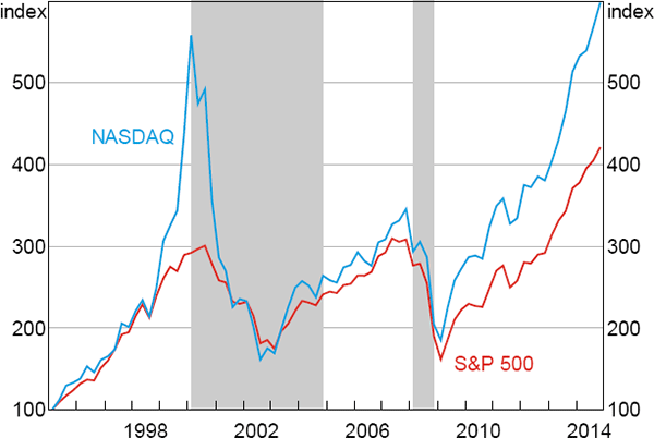
Sources: Authors' calculations; Bloomberg
Our model is silent about the process through which agents infer changes in steady-state productivity growth. Nevertheless, our results are consistent with those of a standard learning model in which agents have imperfect information about the true structure of the economy, including the steady-state rate of productivity growth, and so continuously update their beliefs about the structure from the behaviour of observable variables. To illustrate this, we estimate a simple model in which agents update their beliefs about the reduced form structure of the economy by regressing a set of observable variables, Yt, on a set of exogenous regressors, Xt. We assume that agents form beliefs using a constant-gain algorithm, implying that they place a greater weight on more recent observations.
To fix notation, let Yt denote a vector of observable variables consisting of GDP growth, consumption growth, real wage growth and the change in a long-term real interest rate, Yt = (Δyt, Δct, Δwt, Δ(rt − Etπt + 1)).[10] We include these variables because they are likely to provide useful information about steady-state productivity growth. In standard models output, consumption and real wages will in steady state grow at the same rate as TFP growth, while the change in the real interest rate will be zero. As exogenous regressors, Xt, we include a constant and three lags of each of the endogenous variables. Let ωt be the vector of estimated reduced form coefficients at time t. Then, using data through period t, the parameters for the constant-gain least squares learning model evolve according to the algorithm:
where Ω is the covariance matrix of the reduced-form coefficients. The parameter κ is the gain, which governs the extent to which agents discount the past when updating their coefficient estimates. We set κ = 0.015, which is around the middle of the estimates of this parameter used in the literature (Orphanides and Williams 2005; Milani 2007, 2008; Slobodyan and Wouters 2012).[11] We estimate the model over the period 1953:Q3 to 2014:Q4.
Figure 10 shows the evolution of the estimated long-run mean values of each of the endogenous regressors. This is equivalent to the time-varying steady state of the estimated system of equations. To compare these results to our main estimates, we also plot the 90 per cent confidence interval for initial steady-state TFP growth from our estimated business cycle model, as documented in Table 1.
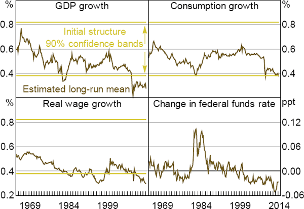
Recall that in the DSGE model output, consumption and real wages all grow at the same rate as TFP in steady state. Using a completely different approach, the learning model described here produces results that are strongly consistent with the DSGE evidence. Specifically, until the early 2000s, the estimated long-run means of output and consumption growth for the most part lie within the 90 per cent confidence bands of the DSGE model's estimates of steady-state TFP growth. The evidence for real wages is not as strong, although even here the parameter estimate lies within the 90 per cent confidence bands for much of the time. Similarly, the estimated long-run value of the change in the real interest rate is close to zero, consistent with stable expectations about steady-state TFP growth.
More recently, the estimated long-run means of output and real wages growth have drifted well below the DSGE model's estimate of the US economy's initial steady-state TFP growth rate. The long-run mean of consumption growth has also drifted to the bottom of the 90 per cent confidence band. The estimated long-run value of output and real wages growth reached a level consistent with the DSGE model's estimate of the final rate of steady-state TFP growth, although the long-run mean of consumption growth remained somewhat above that level. At the same time, the estimated long-run mean of the real interest rate has declined below zero, as one would expect if there were a decline in agents' beliefs about steady-state TFP growth. The timing of the downward shift in these long-run means coincides remarkably closely with the estimated break in beliefs about steady-state TFP growth in the DSGE model.
4.1.3 Why not the 1990s?
The late 1990s was a time of strong productivity growth in the United States. A number of papers identify an increase in trend productivity growth at this time (e.g. Kahn and Rich 2007; Fernald 2014). Why does the model identify a slowdown in trend growth before this episode, and why does it not identify a pick-up in productivity growth at this time?
Again, it is informative to inspect the model's productivity data. Figure 11 compares the model's estimates of productivity growth during the 1990s against Fernald's (2014) estimates. The two series differ more in this decade than they did during the 1970s, although the correlation is still 0.62. More importantly, both series identify strong productivity growth outcomes in the late 1990s, consistent with conventional views about this era.
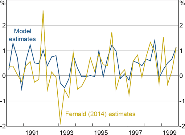
Sources: Authors' calculations; Fernald (2014)
But the strong productivity outcomes of the late 1990s are compatible with a reduction in trend productivity growth in the 1970s. Recall Equation (1)
This specification implies that the economy can receive shocks that temporarily drive productivity growth away from its long-run trend. In theory, these shocks should be serially uncorrelated. But in a sample there may be periods in which a succession of positive shocks occurs. The model suggests that the 1990s was one of those times. Of course, the model may have been able to fit the productivity data in this era with smaller shocks by allowing for a positive increase in trend productivity in the 1990s. The reason it does not identify such a break is that doing so would have worsened the fit of the model along other dimensions. In particular, it would require larger shocks to match the observations in the 2000s.
5. Implications of Lower Productivity Growth
In this section we highlight some of the implications of lower steady-state productivity growth for the US economy.
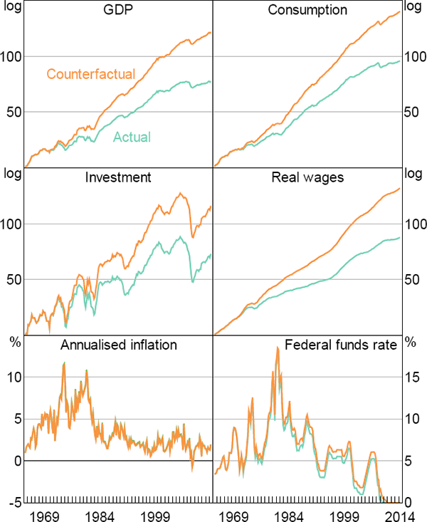
We first focus on how the break in productivity growth has affected the US economy over recent decades. Figure 12 presents counterfactuals that show how economic outcomes would have evolved without the break in productivity growth. The lines marked ‘actual’ show the actual paths of GDP, consumption, investment, real wages, inflation and interest rates since the mid 1960s. The lines marked ‘counterfactual’ adjust the actual path of these variables for the estimated effects of the break in productivity growth, incorporating the delay in the adjustment of beliefs.
Our estimates point to a halving of steady-state productivity growth. Cumulated over three decades, this implies a substantial fall in living standards relative to their counterfactual levels. For instance, the levels of per capita GDP and consumption would both be around 45 per cent higher if productivity growth had not declined. Moreover, our estimation attributes almost all of the stagnation in real wages over recent decades to the slowdown in productivity growth.
Aside from its effects on real variables, the counterfactual exercise also highlights the consequences of the decrease in productivity growth for monetary policy. Counterfactual interest rates tracked the federal funds rate closely until the late 1980s. From that point the two series diverge. By the mid 2000s, the counterfactual federal funds rate is almost 75 basis points above the actual rate. Without the slowdown in productivity growth, US interest rates would not have been nearly so low in the mid 2000s.
The implications are even more significant in the more recent period, in which the Federal Reserve has been constrained by the zero lower bound. The federal funds rate reached its lower bound in 2008:Q4. At that time, the counterfactual federal funds rate was still above 1 per cent. This rate did not reach zero until 2010:Q4. That is, without the slowdown in productivity growth, it appears that the Federal Reserve would have had more room to address the negative consequences of the Great Recession.
Sources: Authors' calculations; Bureau of Economic Analysis; Bureau of Labor Statistics
Looking forward, slower steady-state productivity growth implies a lower neutral real interest rate. For a given inflation target, this implies a lower neutral nominal interest rate. Unless the size of the shocks affecting the US economy become smaller than has been the case over recent decades, this means that the zero lower bound (ZLB) is likely to bind more frequently in the future than has been the case in the past.
To give a sense of the magnitudes, for both the initial and final steady-state productivity growth rates we conducted 10,000 model simulations of 240 quarters, setting all other parameters to their posterior median values. In the simulations we imposed a zero lower bound on nominal interest rates.[12] For each simulation, we record the number of times the nominal interest rate reached zero and the proportion of time the interest rate spends at zero.[13] Table 2 shows the results.
Our estimates suggest that the neutral real interest rate in the United States has fallen from 2.9 per cent before the early 1980s to 1.9 per cent today. Similarly, the neutral nominal interest rate has fallen from 5.5 per cent to 4.4 per cent. In the simulations, lower neutral rates substantially increase the frequency and duration of zero lower bound episodes. The average number of lower bound episodes per simulation increases from 2.5, or one every 25 years, to 4, or one ever 15 years. And the proportion of time spent at the zero lower bound roughly doubles.
| Regime | Neutral real interest rate | Neutral nominal interest rate | Number of ZLB episodes | Proportion of time spent at ZLB | ||
|---|---|---|---|---|---|---|
| Mean | Median | Mean | Median | |||
| Initial (γ= 0.59) | 2.90 | 5.45 | 2.5 | 2.0 | 2.6 | 1.2 |
| Final (γ= 0.33) | 1.86 | 4.39 | 3.9 | 3.0 | 4.7 | 3.2 |
6. Robustness
6.1 Model-based Extensions
So far, we have presented results under the assumption that there has been a single break in US productivity growth and that agents may have failed to observe the break in real time. An alternative hypothesis is that there have been multiple breaks in steady-state productivity growth over our sample. For example, the break that we identify in agents' beliefs about productivity growth may actually represent a further break in steady-state growth. Alternatively, the strong productivity outcomes recorded in the 1990s might indicate that there was an increase in steady-state productivity growth at this time alongside a decrease at another time. To investigate these possibilities, we estimate a model allowing for two breaks in productivity growth.[14]
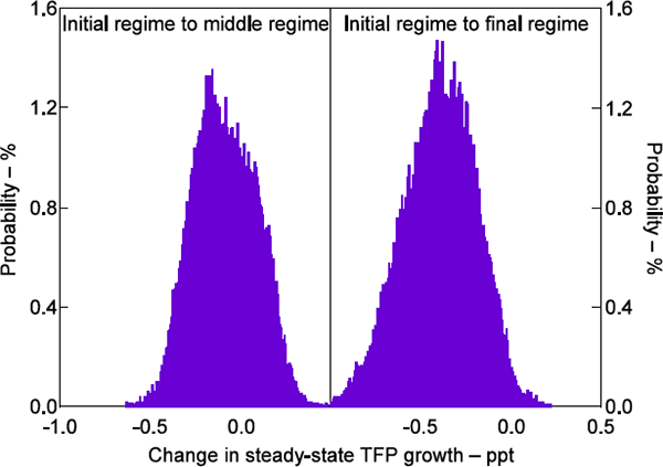
With two breaks in productivity growth we allow for three productivity regimes, an initial, a middle and a final regime. Figure 13 shows the estimated change in steady-state productivity growth between the initial regime and the middle regime (left panel) and the initial regime and the final regime (right panel). Clearly, the estimation struggles to identify more than a single break in TFP growth – the estimate of productivity growth in the middle regime is about as likely be larger than productivity growth in the initial regime as it is to be smaller. In contrast, there is a high probability that productivity growth in the final regime was lower than in the initial regime. The difference in productivity between the initial and final regime is also broadly in line with our baseline results. Overall, a single break appears to be sufficient to account for changes in productivity over our estimation sample.
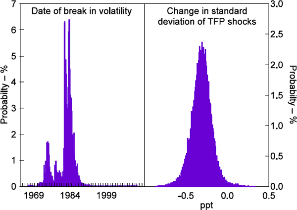
Our estimation sample spans the period before and after the start of the ‘Great Moderation’, when the volatility of many US macroeconomic series declined noticeably. One might wonder whether the shifts in productivity growth that we estimate might actually be accounting for time variation in the variance of productivity. To explore this possibility, we re-estimate our preferred model allowing for a break in the variance of productivity shocks. As one might expect, we find strong evidence that the variance of productivity shocks declined in the early 1980s (Figure 14). But allowing for a break in the variance of productivity growth has little effect on the estimated timing or magnitude of the break in steady-state productivity growth.
In estimation, we used a single measure of wages growth – hourly compensation of employees. In this regard we depart from the approach of Justiniano et al (2013), who use the same model as ours but in estimation include an additional observable wage series – average hourly earnings of non-supervisory employees. Figure 15 summarises our main results when we estimate our model using the same observable series as Justiniano et al (2013).
Including an additional observable wage series does not alter our inferences regarding the size of the change in steady-state productivity growth (left panel). If anything, the estimated probability that steady-state productivity growth has fallen is slightly larger in this specification. Moreover, our estimates of initial and final steady-state productivity growth are also largely unaffected.
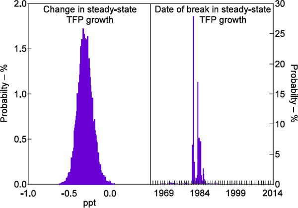
However, our estimates of the date at which productivity growth decreased shift by around a decade, to the early 1980s.[15] We find it difficult to rationalise a break at this date. As we discuss in greater detail in Appendix F, we suspect that the estimation may be using the break to account for the lower mean of the hourly earnings series relative to the compensation series. This lower mean is likely, in part, to reflect the fact that the coverage of the hourly earnings series is less representative of the US workforce than the compensation series. As we do not want these compositional issues to affect our estimates it is appropriate to exclude this series from our baseline specification.
We have also experimented with alternative specifications that include: increasing the number of breaks allowed in estimation, adding long-term interest rates (which may contain information about expectations of future productivity growth) as additional observable variables and allowing agents to anticipate future shifts in steady-state productivity growth. All of these cases support our core findings of a decrease in steady-state productivity growth in the early 1970s and an adjustment of agents' beliefs about steady-state productivity growth some decades after that.
6.2 Other Considerations
There are a number of other issues that, while not amenable to formal econometric analysis in our model, warrant discussion and investigation in future work.
Since the mid 1980s, the labour share of income in the United States has fallen substantially (Elsby, Hobijn and Şahin 2013). A number of competing explanations for this development exist. These include: a fall in the relative price of information technology-related goods that has led firms to substitute labour for capital (Karabarbounis and Neiman 2014); a decrease in trade unionisation (Elsby et al 2013); rising housing costs (Rognlie 2015); and increased import penetration (Autor, Dorn and Hanson 2013; Elsby et al 2013).
Changes in steady-state productivity growth have only small, temporary effects on the labour share in our model. Therefore, the model attributes changes in factor shares to other structural shocks. Nevertheless, it is notable that the start of the decline in the labour share occurred shortly after the break that we identify in steady-state productivity growth. As discussed above, our identification of this break rests in large part on the behaviour of real wages.
Given the lack of consensus on the cause of the changes in factor shares observed in the United States over recent decades, we are hesitant to say whether allowing for these changes would affect our result. Our sense is that, as the break that we identify occurs prior to the large decrease in the labour share, our results are likely to be robust to such extensions. However, this is ultimately an empirical question. A particularly promising avenue for future research, given the results presented in Rognlie (2015), would be to incorporate a housing sector in the model. Understanding how changes in steady-state productivity growth affect relative housing costs, and how these developments relate to agents' beliefs about future productivity growth would be an interesting question in its own right.
Our results also raise the question of what factors and mechanisms may have prompted the decrease in steady-state productivity growth that we identify. Answering this question is beyond the scope of our model, which is designed to capture the effects of productivity growth rather than its determinants. However, the fact that we identify a break in growth in the early 1970s cautions against explanations that rely heavily on recent economic developments. For instance, a number of authors have argued that the US economy's weak productivity growth in recent years is due in part to the collapse in housing prices that occurred in the late 2000s (e.g. Fort et al 2013). They argue that this development reduced the supply of young businesses, as the owners of these firms often rely on home equity as a source of collateral and to establish credit lines. While this mechanism may well have affected US productivity outcomes in recent years, our results indicate that longer-term factors have also been important.
7. Summary and Conclusion
We estimate a business cycle model of the US economy allowing for breaks in steady-state productivity growth. We find that the pace of steady-state productivity growth halved, most likely in the early 1970s. But this structural break was hard to identify in real time. The behaviour of households and firms indicates that their beliefs about steady-state productivity growth adjusted only in the 2000s.
Finding a break in steady-state productivity growth in the early 1970s is at odds with much of the recent literature, which has tended to identify breaks in the 2000s. Unlike previous work, however, our inferences are based on the behaviour of multiple data series and grounded in economic theory. The use of multiple data series is important because shifts in steady-state productivity growth have implications for the co-movement of many macroeconomic variables. We exploit this information to identify these shifts. And structural estimation is important because agents' beliefs about steady-state productivity growth can differ from reality. The failure of agents to identify shifts in steady-state productivity growth correctly alters the magnitude, and in some cases even the direction, of the responses of macroeconomic variables to these shifts in ways that cannot be gauged without the aid of an economic model.
Looking forward, our results suggest that the average growth rate of the US economy is likely to be considerably lower in the future than was the case for most of the post-war era. Of course, as was the case in the 1990s, there may be periods of unusually rapid technological innovation that provide a temporary boost to growth. But there may also be periods of stagnation, in which growth falls short of even its new lower average.
This paper has focused on the United States. But recent years have seen periods of weak productivity growth in other advanced economies, including the United Kingdom and Australia. And, as in the United States, short-term interest rates in many advanced economies have been at historically low levels since at least 2009. Whether these outcomes reflect transitory factors or shared slowdowns in steady-state productivity growth is an open question that future work could usefully address.
Appendix A: Data Sources
The data construction in Table A1 follows Justiniano et al (2013).
| Series | Source | Other information |
|---|---|---|
| Real GDP | BEA/Federal Reserve Bank of St. Louis | FRED reference GDPC96, cv, sa |
| Implicit price deflator for GDP | BEA/Federal Reserve Bank of St. Louis | FRED reference GDPDEF, sa |
| Personal consumption expenditure | BEA/Federal Reserve Bank of St. Louis | FRED reference PCEC, cv, sa |
| Fixed private investment | BEA/Federal Reserve Bank of St. Louis | FRED reference FPI, cv, sa |
| Civilian employment | BLS/ Federal Reserve Bank of St. Louis | FRED reference CE16OV, sa |
| Civilian non-institutional population | BLS/ Federal Reserve Bank of St. Louis | FRED reference CNP16OV, sa |
| Average weekly hours worked | BLS/ Federal Reserve Bank of St. Louis | FRED reference PRS85006023, sa |
| Hourly compensation of employees | BLS/ Federal Reserve Bank of St. Louis | FRED reference COMPNFB, sa |
| Federal funds rate | Board of Governors of the Federal Reserve System | Statistical release ‘Selected Interest Rates – H.15’ |
| Shadow federal funds rate | Wu and Xia (2014) | Available at <www.frbatlanta.org/cqer/research/shadow_rate.aspx> |
Appendix B: Model Equations
This section documents the log-linearised model equations. The full nonlinear model is described in Justiniano et al (2013).
Production function
Cost minimisation
Phillips curve
Marginal costs
Consumption
Capital utilisation
Value of capital
Investment Euler equation
Capital used in production
Capital accumulation
Aggregate resource constraint
Wage gap
Wage Phillips curve
Taylor rule
GDP
Technology
Exogenous spending
Labour supply
Wage mark-up
Investment-specific TFP shock
Price mark-up shock
Intertemporal shock
Inflation target shock
Year-ended inflation
Measurement equations
Appendix C: Additional Estimation Results
Table C1 documents the estimates of the values of the parameters other than those related to productivity growth for our main model.
| Parameter | Description | Prior | Posterior | |||||
|---|---|---|---|---|---|---|---|---|
| Distribution | Mean | Std error | Mean | Median | 5% | 95% | ||
| α | Capital share | N | 0.30 | 0.05 | 0.17 | 0.17 | 0.16 | 0.18 |
| ιp | Price indexation | B | 0.50 | 0.15 | 0.09 | 0.08 | 0.03 | 0.16 |
| ιw | Wage indexation | B | 0.50 | 0.15 | 0.21 | 0.21 | 0.12 | 0.30 |
| h | Habit formation | N | 0.60 | 0.10 | 0.83 | 0.83 | 0.77 | 0.87 |
| λp | Steady-state price mark-up | N | 0.15 | 0.05 | 0.32 | 0.32 | 0.25 | 0.39 |
log |
Steady-state log hours | N | 0.00 | 0.50 | –0.01 | –0.01 | –0.06 | 0.04 |
100( |
Steady-state inflation | N | 0.63 | 0.10 | 0.63 | 0.63 | 0.46 | 0.79 |
100 |
Discount factor | G | 0.25 | 0.10 | 0.13 | 0.13 | 0.06 | 0.21 |
| ν | Inverse Frisch | G | 2.00 | 0.75 | 2.36 | 2.27 | 1.18 | 3.70 |
| ξp | Price stickiness | B | 0.66 | 0.10 | 0.86 | 0.86 | 0.80 | 0.93 |
| ξw | Wage stickiness | B | 0.66 | 0.10 | 0.73 | 0.73 | 0.62 | 0.82 |
| χ | Elasticity utility cost | G | 5.00 | 1.00 | 5.18 | 5.12 | 3.42 | 6.97 |
| Spp | Investment-adjusted costs | G | 4.00 | 1.00 | 4.57 | 4.53 | 3.45 | 5.80 |
| ϕπ | Reaction inflation | N | 1.70 | 0.30 | 2.06 | 2.06 | 1.69 | 2.45 |
| ϕy | Reaction GDP growth | N | 0.40 | 0.30 | 1.15 | 1.15 | 0.87 | 1.42 |
| ρR | Auto monetary policy | B | 0.60 | 0.20 | 0.79 | 0.79 | 0.74 | 0.83 |
| ρg | Auto spending | B | 0.60 | 0.20 | 0.99 | 0.99 | 0.99 | 1.00 |
| ρφ | Auto labour supply | B | 0.60 | 0.20 | 0.98 | 0.98 | 0.96 | 0.99 |
| ρμ | Auto investment | B | 0.60 | 0.20 | 0.64 | 0.65 | 0.51 | 0.75 |
| ρp | Auto price mark-up | B | 0.60 | 0.20 | 0.84 | 0.88 | 0.60 | 0.95 |
| ρb | Auto intertemporal | B | 0.60 | 0.20 | 0.49 | 0.49 | 0.34 | 0.65 |
| 100σr | Std dev monetary policy | IG | 0.15 | 1.00 | 0.23 | 0.23 | 0.21 | 0.26 |
| 100σg | Std dev spending | IG | 0.50 | 1.00 | 0.37 | 0.36 | 0.33 | 0.40 |
| 100σφ | Std dev labour supply | IG | 1.00 | 1.00 | 3.26 | 3.09 | 1.65 | 5.27 |
100 |
Std dev wage mark-up | IG | 0.15 | 1.00 | 0.39 | 0.38 | 0.35 | 0.43 |
| 100σμ | Std dev investment | IG | 0.50 | 1.00 | 8.54 | 8.44 | 6.40 | 10.97 |
| 100σp | Std dev price mark-up | IG | 0.15 | 1.00 | 0.08 | 0.07 | 0.06 | 0.10 |
| 100σp | Std dev intertemporal | IG | 0.10 | 1.00 | 0.05 | 0.05 | 0.03 | 0.08 |
100 |
Std dev inflation target | IG | 0.05 | 0.04 | 0.04 | 0.04 | 0.02 | 0.06 |
| Marginal data density: −1,236.7 | ||||||||
|
Note: U denotes uniform distribution, N denotes normal distribution, B denotes beta distribution, G denotes gamma distribution, and IG denotes inverse gamma distribution |
||||||||
Appendix D: Can Our Estimation Recover Date Breaks?
In this appendix, we show that our estimation can identify the timing and magnitude of changes in steady-state productivity growth.
We simulate the model for 201 quarters, with all parameter values set to the posterior means recorded in Justiniano et al (2013). We impose a break in the steady-state growth rate of productivity in quarter 50 that lowers the value of this parameter by 0.4 percentage points, from 0.49 to 0.09. We set the date at which agents' beliefs about steady-state productivity growth adjust to quarter 125. We then estimate our model on the simulated data, using the methodology and priors described in Section 3.
Table D1 shows the estimation results for the parameters of the productivity process and the timing of the structural breaks. The estimation successfully recovers the steady-state productivity growth rates in the initial and final regimes as well as the timing of the break in productivity growth. It also comes very close to matching the persistence of the AR(1) growth process and the standard deviation of productivity shocks. The estimate of the timing of the break in beliefs is slightly less precisely estimated and contains some mass at dates before the actual break. However, the mode and the median of the distribution are both close to the actual break date. Overall, these results give us confidence that the estimation can accurately recover the timing and size of breaks in steady-state productivity growth.
| Parameter | Description | Actual | Posterior | |||
|---|---|---|---|---|---|---|
| Mean(a) | Median | 5% | 95% | |||
| Timing of structural breaks | ||||||
| Tγ | TFP break | 50 | 50 | 50 | 46 | 58 |
| Tb | Beliefs adjust | 125 | 130 | 116 | 59 | 138 |
| TFP breaks | ||||||
| γi | Initial steady-state TFP growth | 0.49 | 0.49 | 0.49 | 0.45 | 0.53 |
| γf | Final steady-state TFP growth | 0.09 | 0.09 | 0.09 | 0.01 | 0.17 |
| ρz | Auto TFP growth | 0.13 | 0.18 | 0.18 | 0.09 | 0.28 |
| 100σz | Std dev TFP growth | 0.87 | 0.81 | 0.81 | 0.74 | 0.89 |
|
Note: (a) Mode reported for the timing of structural breaks |
||||||
Appendix E: The Posterior Sampler
To simulate from the joint posterior of the structural parameters and the date breaks,  ,
we use the Metropolis-Hastings algorithm following a strategy similar to Kulish et
al (2014). As we have continuous and discrete parameters we modify the standard set-up for
Bayesian estimation of DSGE models. We separate the parameters into two blocks: date breaks and
structural parameters. To be clear, though, the sampler delivers draws from the joint posterior
of both sets of parameters.
The first block of the sampler is for the date breaks, T. As is common in the literature on structural breaks (Bai and Perron 1998), we restrict the domain of the date breaks to exclude the first and last 5 per cent of observations. Within the feasible range, we draw from a uniform proposal density and randomise which particular date break in T to update. This approach is motivated by the randomised blocking scheme developed for DSGE models in Chib and Ramamurthy (2010).
The algorithm for drawing for the date breaks block is as follows: We first set initial values of the date breaks, T0, and the structural parameters, ϑ0. Then, for the jth iteration we:
- randomly sample which date breaks to update from a discrete uniform distribution, with support ranging from one to the total number of breaks. For our preferred model this is two.
-
randomly sample the corresponding elements of the proposed date breaks,
 , from a discrete uniform distribution
[Tmin, Tmax] and
set the remaining elements to their values in Tj −
1.
-
calculate the acceptance ratio
 .
.
-
accept the proposal with probability
 setting
  , or Tj −
1 otherwise.
The second block of the sampler is for the nϑ structural parameters. It follows a similar strategy to the date breaks block described above. We randomise over the number and which parameters to possibly update at each iteration. The proposal is a multivariate Student's t distribution.[16] Once again, for the jth iteration we proceed as follows.
-
Randomly sample the number of structural parameters to update from a discrete uniform
distribution
 .
.
-
Randomly sample without replacement which parameters to update from a discrete
uniform distribution
 .
.
-
Construct the proposed
 by drawing the parameters to
update from a multivariate Student's t-distribution with 10 degrees of freedom
and with location set at the corresponding elements of θj − 1. We scale the
draws based on the corresponding elements of the negative inverse Hessian at the posterior
mode.
-
Calculate the acceptance ratio
 .
We set
  if the proposed
  includes inadmissible values (e.g. a proposed negative
value for the standard deviation of a shock) preventing the calculation of
  .
.
-
Accept the proposal with probability
 setting
  , or
, or  otherwise.
We use this multi-block algorithm to construct a chain of 500,000 draws from the joint posterior
 ,
discarding the first 25 per cent as burn-in.
Appendix F: Including Multiple Observed Wage Series in Estimation
Our baseline model includes a single observed wage series – hourly compensation in the total economy. In contrast, Justiniano et al (2013) (whose approach we follow closely) use an additional wage series – average hourly earnings of production and non-supervisory employees – and include measurement error to account for the observed differences between the two series. When we estimate our model using this series we continue to find strong evidence of a break in steady-state productivity growth, and of a substantial gap between the break occurring and agents' expectations adjusting. However, the size of the break is somewhat larger, and it occurs around 10 years later, than in our baseline model. In this appendix, we explain our decision to include only a single observed wage series.
Over our estimation sample, the mean of the two wage series is substantially different.[17] The mean of the hourly compensation series is 1.25 per cent in quarterly terms compared to 1.05 per cent for the hourly earnings series. The differences are even more striking after accounting for inflation – the earnings data imply that real wages did not increase at all between 1973 and 1996, while according to the compensation series, real wages increased by around 25 per cent.
Including the earnings series as an additional observable variable alters the estimation results in three ways. First, as Justiniano et al (2013) note, it reduces the estimated standard deviation of the model's wage mark-up shocks, implying a smaller trade-off between stabilising inflation and stabilising the output gap. Second, it reduces the estimated inflation target. In our baseline model, the mean of the estimated inflation target is 0.63 per cent in quarterly terms. When we include earnings as an observable variable this parameter decreases to 0.28 per cent.
To understand why the inclusion of earnings lowers the estimated inflation target, consider the following decomposition of the growth of nominal wages:
where  is the growth rate of nominal wages,
  is
the steady-state growth rate of real wages,
  is the
steady-state inflation target,
  is the growth rate of the
deviation of nominal wages from their steady state. A lower estimated inflation target allows
the model to match the low observed growth rate of hourly earnings with smaller deviations of
nominal wage growth from its steady state.[18]
The third way in which including the earnings series as an additional observable variable affects the result is by shifting the estimated date of the break in steady-state TFP growth from the early 1970s to the early 1980s. This shift helps the model to match the observed path of real earnings which, after stagnating during the 1970s, decreased during the 1980s.
We find the results for the model that does not include the earnings series as an observable variable to be more plausible. Taken literally, the model that includes earnings implies that the Federal Reserve has an inflation target of just 1 per cent in annualised terms and that inflation has been above target for almost the entire estimation sample, including for much of the period since 2008. This is at odds with most descriptions of Federal Reserve policy over recent decades. The date of the break in steady-state productivity growth in the model that includes earnings is also difficult to reconcile with the observed behaviour of productivity. Moreover, as Champagne et al (2016) discuss, the earnings measure restricts coverage to a particular group of workers whose average earnings have grown less than those of the rest of the US workforce. It therefore may be an undesirable series to use to uncover trends in long-run growth.
References
Autor DH, D Dorn and GH Hanson (2013), ‘The China Syndrome: Local Labor Market Effects of Import Competition in the United States’, The American Economic Review, 103(6), pp 2121–2168.
Bai J and P Perron (1998), ‘Estimating and Testing Linear Models with Multiple Structural Changes’, Econometrica, 66(1), pp 47–78.
Benati L (2007), ‘Drifts and Breaks in Labor Productivity’, Journal of Economic Dynamics & Control, 31(8), pp 2847–2877.
Champagne J, A Kurmann and J Stewart (2016), ‘Reconciling the Differences in Aggregate U.S. Wage Series’, Bank of Canada Staff Working Paper 2016-1.
Chib S and S Ramamurthy (2010), ‘Tailored Randomized Block MCMC Methods with Application to DSGE Models’, Journal of Econometrics, 155(1), pp 19–38.
Cogley T (2005), ‘How Fast Can the New Economy Grow? A Bayesian Analysis of the Evolution of Trend Growth’, Journal of Macroeconomics, 27(2), pp 179–207.
Dolmas J, B Raj and DJ Slottje (1999), ‘The U.S. Productivity Slowdown: A Peak Through the Structural Break Window’, Economic Inquiry, 37(2), pp 226–241.
Elsby MWL, B Hobijn and A Şahin (2013), ‘The Decline of the U.S. Labor Share’, Brookings Papers on Economic Activity, Fall, pp 1–52.
Fernald JG (2014), ‘Productivity and Potential Output Before, During, and After the Great Recession’, Federal Reserve Bank of San Francisco Working Paper No 2014-15.
Fort TC, J Haltiwanger, RS Jarmin and J Miranda (2013), ‘How Firms Respond to Business Cycles: The Role of Firm Age and Firm Size’, NBER Working Paper No 19134.
Gordon RJ (2000), ‘Does the “New Economy” Measure Up to the Great Innovations of the Past?’, Journal of Economic Perspectives, 14(4), pp 49–74.
Gordon RJ (2012), ‘Is U.S. Economic Growth Over? Faltering Innovation Confronts the Six Headwinds’, NBER Working Paper No 18315.
Gordon RJ (2015), ‘Secular Stagnation: A Supply-Side View’, The American Economic Review, 105(5), pp 54–59.
Greenspan A (2000), ‘Technology and the Economy’, Remarks before the Economic Club of New York, New York, 13 January.
Hansen AH (1939), ‘Economic Progress and Declining Population Growth’, The American Economic Review, 29(1), pp 1–15.
Hoffmann M, MU Krause and T Laubach (2012), ‘Trend Growth Expectations and U.S. House Prices Before and After the Crisis’, Journal of Economic Behaviour & Organization, 83(3), pp 394–409.
Jones C (2015), ‘Unanticipated Shocks and Forward Guidance at the Zero Lower Bound’, Unpublished manuscript, New York University, February.
Justiniano A, GE Primiceri and A Tambalotti (2013), ‘Is There a Trade-Off between Inflation and Output Stabilization?’, American Economic Journal: Macroeconomics, 5(2), pp 1–31.
Kahn JA and RW Rich (2007), ‘Tracking the New Economy: Using Growth Theory to Detect Changes in Trend Productivity’, Journal of Monetary Economics, 54(6), pp 1670–1701.
Karabarbounis L and B Neiman (2014), ‘The Global Decline of the Labor Share’, The Quarterly Journal of Economics, 129(1), pp 61–103.
Kass RE and AE Raftery (1995), ‘Bayes Factors’, Journal of the American Statistical Association, 90(430), pp 773–795.
Kulish M, J Morley and T Robinson (2014), ‘Estimating DSGE Models with Forward Guidance’, UNSW Business School Research Paper No 2014 ECON32A.
Kulish M and A Pagan (forthcoming), ‘Estimation and Solution of Models with Expectations and Structural Changes’, Journal of Applied Econometrics.
Luo S and R Startz (2014), ‘Is it One Break or Ongoing Permanent Shocks that Explains U.S. Real GDP?’, Journal of Monetary Economics, 66, pp 155–163.
Milani F (2007), ‘Expectations, Learning and Macroeconomic Persistence’, Journal of Monetary Economics, 54(7), pp 2065–2082.
Milani F (2008), ‘Learning, Monetary Policy Rules, and Macroeconomic Stability’, Journal of Economic Dynamics & Control, 32(10), pp 3148–3165.
Orphanides A and JC Williams (2005), ‘The Decline of Activist Stabilization Policy: Natural Rate Misperceptions, Learning, and Expectations’, Journal of Economic Dynamics & Control, 29(11), pp 1927–1950.
Perron P and T Wada (2009), ‘Let's Take a Break: Trends and Cycles in US Real GDP’, Journal of Monetary Economics, 56(6), pp 749–765.
Reifschneider D, W Wascher and D Wilcox (2015), ‘Aggregate Supply in the United States: Recent Developments and Implications for the Conduct of Monetary Policy’, IMF Economic Review, 63(1), pp 71–109.
Rognlie M (2015), ‘Deciphering the Fall and Rise in the Net Capital Share: Accumulation or Scarcity?’, Brookings Papers on Economic Activity, Spring, pp 1–54.
Slobodyan S and R Wouters (2012), ‘Learning in an Estimated Medium-Scale DSGE Model’, Journal of Economic Dynamics & Control, 36(1), pp 26–46.
Smets F and R Wouters (2007), ‘Shocks and Frictions in US Business Cycles: A Bayesian DSGE Approach’, The American Economic Review, 97(3), pp 586–606.
Summers LH (2014), ‘U.S. Economic Prospects: Secular Stagnation, Hysteresis, and the Zero Lower Bound’, Business Economics, 49(2), pp 65–73.
Summers LH (2015), ‘Demand Side Secular Stagnation’, The American Economic Review, 105(5), pp 60–65.
Wu JC and FD Xia (2014), ‘Measuring the Macroeconomic Impact of Monetary Policy at the Zero Lower Bound’, NBER Working Paper No 20117.
Acknowledgements
We would like to thank Heather Anderson, John Simon, Greg Kaplan, Peter Tulip, Mariano Kulish, Christopher Gibbs, Jarkko Jääskelä and participants at seminars at the Reserve Bank of Australia and the Melbourne Institute Macroeconomic Policy Meeting for helpful comments and suggestions. The views expressed in this paper are those of the authors and do not necessarily reflect those of the Reserve Bank of Australia. The authors are solely responsible for any errors.
Footnotes
For example, see Graph 1 of Reifschneider, Wascher and Wilcox (2015). [1]
In most economic models, TFP growth is the only source of long-run growth in output per capita. [2]
This demand-side explanation appears closer in spirit to the original description of secular stagnation by Hansen (1939), although more recently the term has come to refer to both demand-side and supply-side explanations for slower growth. [3]
Appendix D documents the results of this exercise. [4]
The wage series we use is the Bureau of Economic Analysis' (BEA) hourly compensation of employees series. Justiniano et al (2013) use an additional wage series, the Bureau of Labor Statistics' (BLS) average hourly earnings of non-supervisory employees series, in estimation. In Appendix F we explain why we exclude this series. [5]
Examples of estimated DSGE models that take account of the zero lower bound include Kulish, Morley and Robinson (2014) and Jones (2015). [6]
We also experimented with a lower prior mean for γi and γf. This modification has almost no effect on our results. [7]
In Section 6, we show that this conclusion holds even when we allow for multiple breaks in productivity growth. [8]
Our estimation differs from Justiniano et al (2013) in two dimensions: we allow for a break in productivity growth and we have an additional five years of data. To test whether the discrepancies that we find in the parameter estimates are due to having additional data we estimated a model with our full data series but without allowing for a break in productivity growth. These results suggest that most of the differences in parameter estimates – other than those related to productivity growth – between our main results and those in Justiniano et al are due to the longer data sample. [9]
For the real interest rate, we subtract the Survey of Professional Forecasters' one-year-ahead inflation expectations from the 10-year constant maturity bond yield. We also experimented with using the level of real interest rates rather than the change. For much of the sample, this specification produced similar results to those documented in the text. However, it produced unstable parameter estimates during the period of rapidly increasing long-term bond yields associated with the Volcker disinflation. [10]
Small changes in κ, varying the lag length or excluding individual variables all make almost no difference to our results. [11]
We imposed the lower bound using the techniques described in Kulish et al (2014) and Jones (2015). In addition to imposing the zero lower bound constraint period-by-period, these techniques also account for the fact that agents may expect the zero lower bound to bind in future periods. [12]
We classify a zero lower bound episode as one in which the interest rate reaches the lower bound for the first time in at least eight quarters. That is, we categorise episodes in which the interest rate shifts from the lower bound to a positive value for just a few quarters before returning to zero as a single lower bound episode. [13]
In this exercise we assume that agents observe the break when it occurs. [14]
The estimated date of the break in agents' beliefs about steady-state productivity growth are similar to our baseline specification. [15]
We compute the Hessian of the proposal density at the mode of the structural parameters. [16]
Champagne, Kurmann and Stewart (2016) discuss the conceptual differences between alternative US wage measures. [17]
Of course, this also implies larger deviations of inflation from its steady state. However, because of the persistence of the model's inflation target shock, the model requires relatively small shocks to achieve this path of inflation. [18]


