RDP 2016-08: The Slowdown in US Productivity Growth: Breaks and Beliefs 4. Results
October 2016
- Download the Paper 1.59MB
In this section we present results for our preferred model, which features a single break in steady-state productivity growth and allows agents' beliefs about steady-state productivity growth to change at a different date to the actual break. In Section 6, we compare these results to alternative specifications.
The left panel of Figure 4 shows the probability density function (PDF) of the posterior distribution of the timing of the break in steady-state productivity growth. The estimation strongly prefers a break in productivity growth in the early 1970s – the mode of the distribution occurs in 1970:Q4 and the median around one year later. The estimation assigns a small probability to the break occurring in the 2000s. But it has little mass in the 1990s, indicating that the model does not interpret the pick-up in productivity growth at this time as a shift in steady-state productivity growth.[8]
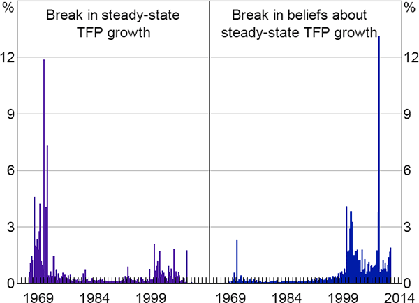
The right panel of Figure 4 shows the PDF of the date at which agents' beliefs about productivity growth changed. The results indicate that the shift in agents' beliefs about steady-state productivity growth occurred well after the actual break. There is substantial mass in the early 2000s, although the mode of the distribution is a bit later, in 2008.
Table 1 documents the estimation results for the remaining parameters of the productivity growth process. The point estimate of the initial steady-state TFP growth rate, γi = 0.59, is slightly higher than reported in other structural models of the US economy (for example, Justiniano et al (2013), which was 0.47, and Smets and Wouters (2007), which was 0.43), although the 90 per cent confidence interval spans these earlier estimates. The estimation points to a large slowdown in steady-state productivity growth after the structural break. In fact, the point estimates suggest that quarterly steady-state productivity growth has almost halved from 0.59 per cent to 0.33 per cent. The estimates of the persistence of the TFP process, ρz, and the standard deviation of shocks to productivity growth, σz, are similar to those reported in Justiniano et al (2013).
| Parameter | Description | Prior | Posterior | |||||
|---|---|---|---|---|---|---|---|---|
| Distribution | Mean | Std error | Mean(a) | Median | 5% | 95% | ||
| Timing of structural breaks | ||||||||
| Tγ | TFP break | U | [1965:Q3–2012:Q1](b) | 1970:Q4 | 1971:Q4 | 1981:Q2 | 1986:Q1 | |
| Tb | Beliefs adjust | U | [1965:Q3–2012:Q1](b) | 2008:Q4 | 2003:Q1 | 1997:Q2 | 2011:Q3 | |
| TFP process | ||||||||
| γi | Initial growth | N | 0.50 | 0.20 | 0.59 | 0.58 | 0.38 | 0.82 |
| γf | Final growth | N | 0.50 | 0.20 | 0.33 | 0.34 | 0.14 | 0.47 |
| ρz | Auto TFP | B | 0.40 | 0.20 | 0.06 | 0.06 | 0.01 | 0.14 |
| 100σz | Std dev TFP | IG | 1.00 | 1.00 | 0.90 | 0.90 | 0.82 | 0.99 |
| Marginal data density: −1,236.7 | ||||||||
|
Notes: U denotes uniform distribution, N denotes normal distribution, B denotes
beta distribution, and IG denotes inverse gamma distribution |
||||||||
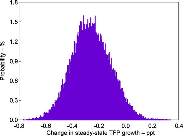
Our finding of a slowdown in steady-state productivity growth is economically meaningful. But is it statistically so? We present two pieces of evidence to suggest that it is. First, Figure 5 shows the posterior distribution of the change in productivity growth between the initial and final steady states. To construct this figure we compute the difference between the final steady-state productivity growth rate and the initial rate (that is, (γf − γi) for each draw from the posterior distribution and plot the histogram of these values. The 90 per cent highest probability interval for this distribution spans −0.49 to −0.01. That is, the estimation finds little evidence that the steady-state productivity growth rate has increased or even stayed the same.
Second, we re-estimated the model without allowing for a structural break in TFP growth (or beliefs about TFP growth). The marginal data density of our baseline model is −1,236.7. The marginal data density of the no-breaks model is −1,238.4. A standard metric for model comparison is twice the log Bayes factor, which in this case is equal to 3.3. Using the criteria of Kass and Raftery (1995), this provides positive evidence in favour of a model that allows for a break in productivity growth.
Appendix C contains estimation results for the other parameters of the model. For the most part, these parameter estimates are very close to those reported in Justiniano et al (2013). That is, while we find strong evidence that there has been a slowdown in the steady-state productivity growth rate, ignoring this slowdown does not appear to change the other estimated properties of the model.[9]
4.1 Why Do We Find the Breaks Where We Do?
In this section we discuss why the estimation identifies break dates where it does. We first highlight features of the data that lead the estimation to identify breaks in the 1970s and 2000s. We then discuss why the data does not identify a break in the 1990s, as some previous research has.
4.1.1 Why do we estimate a break in trend productivity growth in the 1970s?
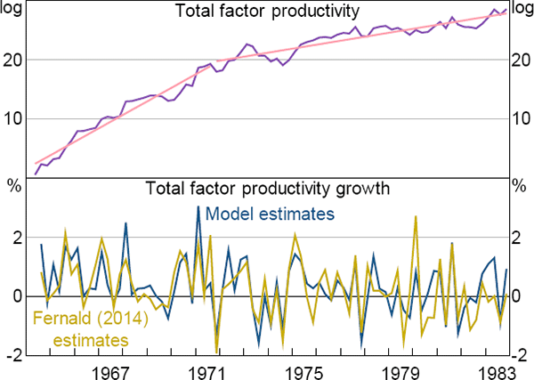
A natural starting point to understand why the estimation identifies a break in steady-state TFP growth in the early 1970s is to look at the behaviour of productivity itself. The top panel of Figure 6 plots the estimated log level of productivity implied by the model (with all parameters set at their posterior median values). The two straight segments plot lines of best fit over the period 1964:Q2 to 1971:Q3 (that is, before the estimated break) and between 1971:Q4 and 1983:Q4 (that is, the 12 years after the estimated break). The slope of the segments clearly declines in the latter period, indicative of a slowdown in average productivity growth.
Sources: Authors' calculations; Fernald (2014)
Of course, productivity cannot be observed directly, and productivity measures may be contaminated by cyclical influences or measurement error. These factors, however, do not appear to be driving the patterns shown in the top panel of Figure 6. To illustrate this, the bottom panel of the figure plots the model's estimated productivity growth series against an alternative series published in Fernald (2014). Fernald constructs a series that accords closely to the theoretical concept of TFP by removing from the official US productivity statistics the effects of variation in the utilisation of capital and labour as well as improvements in the quality of labour. Despite the conceptual differences, our estimates correspond closely to Fernald's series, with a correlation over the sample in the figure of 0.71. Like us, Fernald's series indicates a slowdown in the average pace of productivity growth in the early 1970s.
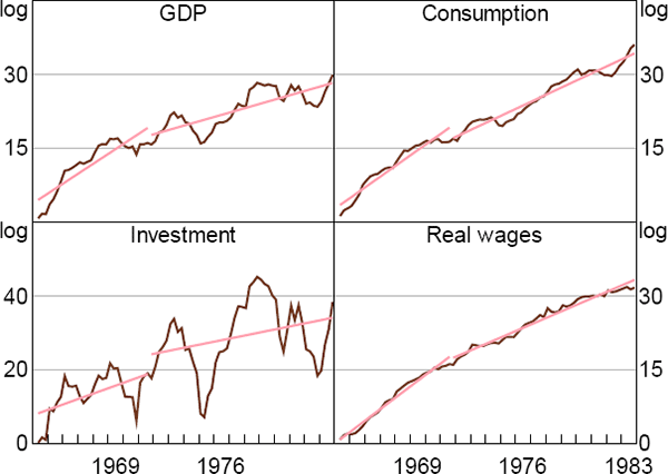
As we emphasised in Section 2, our estimation procedure takes account of the joint behaviour of a range of macroeconomic variables to form inferences about breaks in steady-state productivity growth. Recall from Figure 3 that we should expect a decrease in steady-state productivity growth to lower the growth rates of GDP, consumption, investment and real wages. Figure 7 graphs the evolution of these variables over the period 1964:Q2 to 1983:Q4. As in Figure 6, the straight lines correspond to lines of best fit over the sub-samples 1964:Q2 to 1971:Q3 and 1971:Q4 to 1983:Q4.
Sources: Authors' calculations; Bureau of Economic Analysis; Bureau of Labor Statistics
For all four variables, average growth rates decrease after the estimated break in productivity growth, consistent with the theoretical predictions. The decrease in average consumption growth, however, is modest compared to those of GDP and real wages. This may help to explain why the model assigns little probability to there being a break in agents' beliefs about trend productivity growth at this time.
4.1.2 Why didn't agents perceive the slowdown until the 2000s?
The estimation suggests that beliefs about steady-state productivity growth adjusted in the 2000s, with the periods of greatest probability being 2000–01 and 2008. Both of these date ranges coincided with periods of weak output and consumption growth, consistent with Figure 3. Mechanically, we would expect these patterns to lead the estimation to identify a break in agents' beliefs at these times. But, of course, the recessions of the early 2000s and 2007–09 had a range of causes and one would not attribute them solely to changes in beliefs about future productivity growth. In this section, we show that a downward shift in expectations about future steady-state productivity growth is consistent with the pattern of agents' forecast errors as well as evidence from outside the model.
One reason for scepticism about the three-decade gap that we estimate between the break in steady-state productivity growth and the shift in agents' beliefs is that it seems to imply that households and firms would have made persistent forecast errors for an implausibly long time. It turns out, however, that this is not the case. To illustrate this, Figure 8 plots the cumulative one-step-ahead forecast errors of GDP growth made by agents in the model. The errors account for the fact that, between 1971 and 2003, agents' beliefs about steady-state productivity growth remained at their initial level even though actual steady-state productivity growth had declined.
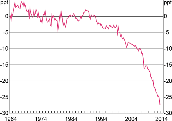
If agents in the model persistently overestimated productivity growth, we would expect to see these cumulative errors become increasingly negative. Such a drift is not apparent until the early 2000s. After that, agents' one-step-ahead forecasts persistently overestimated the actual outcomes of these variables. This pattern of errors is intuitive. As noted above, the 1990s was a time of strong productivity growth in the United States, albeit one that we would argue was driven by temporary factors rather than a permanent shift in steady-state growth. In such an environment, it is natural that agents would have underpredicted future consumption or output growth as often as they would have overpredicted these quantities. Given this pattern of forecast errors, it is understandable that it would take agents many years to revise their beliefs about steady-state productivity growth.
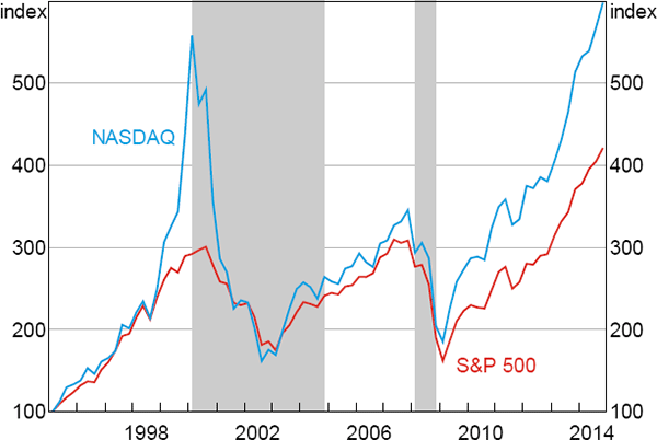
The timing of the shift in agents' beliefs is also consistent with evidence from outside the model. Asset prices are a natural place to look for shifts in beliefs about long-run productivity growth as they should be forward looking and rapidly incorporate new information. Figure 9 plots the NASDAQ and S&P 500 stock market indices over recent decades, with the highlighted areas corresponding to the periods in which our estimation assigns a high probability to beliefs about steady-state productivity growth shifting down. Both periods of high probability coincided with large falls in equity prices, consistent with beliefs about long-run productivity growth declining at these times.
Sources: Authors' calculations; Bloomberg
Our model is silent about the process through which agents infer changes in steady-state productivity growth. Nevertheless, our results are consistent with those of a standard learning model in which agents have imperfect information about the true structure of the economy, including the steady-state rate of productivity growth, and so continuously update their beliefs about the structure from the behaviour of observable variables. To illustrate this, we estimate a simple model in which agents update their beliefs about the reduced form structure of the economy by regressing a set of observable variables, Yt, on a set of exogenous regressors, Xt. We assume that agents form beliefs using a constant-gain algorithm, implying that they place a greater weight on more recent observations.
To fix notation, let Yt denote a vector of observable variables consisting of GDP growth, consumption growth, real wage growth and the change in a long-term real interest rate, Yt = (Δyt, Δct, Δwt, Δ(rt − Etπt + 1)).[10] We include these variables because they are likely to provide useful information about steady-state productivity growth. In standard models output, consumption and real wages will in steady state grow at the same rate as TFP growth, while the change in the real interest rate will be zero. As exogenous regressors, Xt, we include a constant and three lags of each of the endogenous variables. Let ωt be the vector of estimated reduced form coefficients at time t. Then, using data through period t, the parameters for the constant-gain least squares learning model evolve according to the algorithm:
where Ω is the covariance matrix of the reduced-form coefficients. The parameter κ is the gain, which governs the extent to which agents discount the past when updating their coefficient estimates. We set κ = 0.015, which is around the middle of the estimates of this parameter used in the literature (Orphanides and Williams 2005; Milani 2007, 2008; Slobodyan and Wouters 2012).[11] We estimate the model over the period 1953:Q3 to 2014:Q4.
Figure 10 shows the evolution of the estimated long-run mean values of each of the endogenous regressors. This is equivalent to the time-varying steady state of the estimated system of equations. To compare these results to our main estimates, we also plot the 90 per cent confidence interval for initial steady-state TFP growth from our estimated business cycle model, as documented in Table 1.
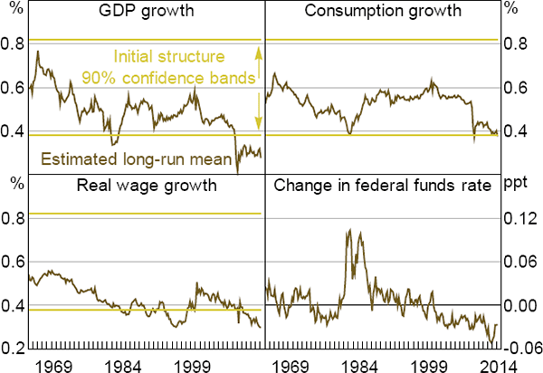
Recall that in the DSGE model output, consumption and real wages all grow at the same rate as TFP in steady state. Using a completely different approach, the learning model described here produces results that are strongly consistent with the DSGE evidence. Specifically, until the early 2000s, the estimated long-run means of output and consumption growth for the most part lie within the 90 per cent confidence bands of the DSGE model's estimates of steady-state TFP growth. The evidence for real wages is not as strong, although even here the parameter estimate lies within the 90 per cent confidence bands for much of the time. Similarly, the estimated long-run value of the change in the real interest rate is close to zero, consistent with stable expectations about steady-state TFP growth.
More recently, the estimated long-run means of output and real wages growth have drifted well below the DSGE model's estimate of the US economy's initial steady-state TFP growth rate. The long-run mean of consumption growth has also drifted to the bottom of the 90 per cent confidence band. The estimated long-run value of output and real wages growth reached a level consistent with the DSGE model's estimate of the final rate of steady-state TFP growth, although the long-run mean of consumption growth remained somewhat above that level. At the same time, the estimated long-run mean of the real interest rate has declined below zero, as one would expect if there were a decline in agents' beliefs about steady-state TFP growth. The timing of the downward shift in these long-run means coincides remarkably closely with the estimated break in beliefs about steady-state TFP growth in the DSGE model.
4.1.3 Why not the 1990s?
The late 1990s was a time of strong productivity growth in the United States. A number of papers identify an increase in trend productivity growth at this time (e.g. Kahn and Rich 2007; Fernald 2014). Why does the model identify a slowdown in trend growth before this episode, and why does it not identify a pick-up in productivity growth at this time?
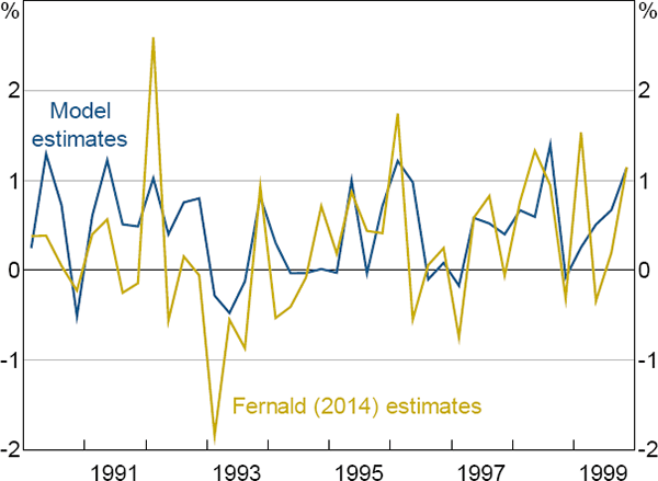
Again, it is informative to inspect the model's productivity data. Figure 11 compares the model's estimates of productivity growth during the 1990s against Fernald's (2014) estimates. The two series differ more in this decade than they did during the 1970s, although the correlation is still 0.62. More importantly, both series identify strong productivity growth outcomes in the late 1990s, consistent with conventional views about this era.
Sources: Authors' calculations; Fernald (2014)
But the strong productivity outcomes of the late 1990s are compatible with a reduction in trend productivity growth in the 1970s. Recall Equation (1)
This specification implies that the economy can receive shocks that temporarily drive productivity growth away from its long-run trend. In theory, these shocks should be serially uncorrelated. But in a sample there may be periods in which a succession of positive shocks occurs. The model suggests that the 1990s was one of those times. Of course, the model may have been able to fit the productivity data in this era with smaller shocks by allowing for a positive increase in trend productivity in the 1990s. The reason it does not identify such a break is that doing so would have worsened the fit of the model along other dimensions. In particular, it would require larger shocks to match the observations in the 2000s.
Footnotes
In Section 6, we show that this conclusion holds even when we allow for multiple breaks in productivity growth. [8]
Our estimation differs from Justiniano et al (2013) in two dimensions: we allow for a break in productivity growth and we have an additional five years of data. To test whether the discrepancies that we find in the parameter estimates are due to having additional data we estimated a model with our full data series but without allowing for a break in productivity growth. These results suggest that most of the differences in parameter estimates – other than those related to productivity growth – between our main results and those in Justiniano et al are due to the longer data sample. [9]
For the real interest rate, we subtract the Survey of Professional Forecasters' one-year-ahead inflation expectations from the 10-year constant maturity bond yield. We also experimented with using the level of real interest rates rather than the change. For much of the sample, this specification produced similar results to those documented in the text. However, it produced unstable parameter estimates during the period of rapidly increasing long-term bond yields associated with the Volcker disinflation. [10]
Small changes in κ, varying the lag length or excluding individual variables all make almost no difference to our results. [11]


