RDP 2016-08: The Slowdown in US Productivity Growth: Breaks and Beliefs Appendix E: The Posterior Sampler
October 2016
- Download the Paper 1.59MB
To simulate from the joint posterior of the structural parameters and the date breaks,  ,
we use the Metropolis-Hastings algorithm following a strategy similar to Kulish et
al (2014). As we have continuous and discrete parameters we modify the standard set-up for
Bayesian estimation of DSGE models. We separate the parameters into two blocks: date breaks and
structural parameters. To be clear, though, the sampler delivers draws from the joint posterior
of both sets of parameters.
,
we use the Metropolis-Hastings algorithm following a strategy similar to Kulish et
al (2014). As we have continuous and discrete parameters we modify the standard set-up for
Bayesian estimation of DSGE models. We separate the parameters into two blocks: date breaks and
structural parameters. To be clear, though, the sampler delivers draws from the joint posterior
of both sets of parameters.
The first block of the sampler is for the date breaks, T. As is common in the literature on structural breaks (Bai and Perron 1998), we restrict the domain of the date breaks to exclude the first and last 5 per cent of observations. Within the feasible range, we draw from a uniform proposal density and randomise which particular date break in T to update. This approach is motivated by the randomised blocking scheme developed for DSGE models in Chib and Ramamurthy (2010).
The algorithm for drawing for the date breaks block is as follows: We first set initial values of the date breaks, T0, and the structural parameters, ϑ0. Then, for the jth iteration we:
- randomly sample which date breaks to update from a discrete uniform distribution, with support ranging from one to the total number of breaks. For our preferred model this is two.
-
randomly sample the corresponding elements of the proposed date breaks,
 , from a discrete uniform distribution
[Tmin, Tmax] and
set the remaining elements to their values in Tj −
1.
, from a discrete uniform distribution
[Tmin, Tmax] and
set the remaining elements to their values in Tj −
1.
-
calculate the acceptance ratio
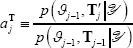 .
.
-
accept the proposal with probability
 setting
  , or Tj −
1 otherwise.
, or Tj −
1 otherwise.
The second block of the sampler is for the nϑ structural parameters. It follows a similar strategy to the date breaks block described above. We randomise over the number and which parameters to possibly update at each iteration. The proposal is a multivariate Student's t distribution.[16] Once again, for the jth iteration we proceed as follows.
-
Randomly sample the number of structural parameters to update from a discrete uniform
distribution
 .
.
-
Randomly sample without replacement which parameters to update from a discrete
uniform distribution .
-
Construct the proposed
 by drawing the parameters to
update from a multivariate Student's t-distribution with 10 degrees of freedom
and with location set at the corresponding elements of θj − 1. We scale the
draws based on the corresponding elements of the negative inverse Hessian at the posterior
mode.
by drawing the parameters to
update from a multivariate Student's t-distribution with 10 degrees of freedom
and with location set at the corresponding elements of θj − 1. We scale the
draws based on the corresponding elements of the negative inverse Hessian at the posterior
mode.
-
Calculate the acceptance ratio
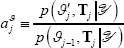 .
We set
.
We set  if the proposed includes inadmissible values (e.g. a proposed negative
value for the standard deviation of a shock) preventing the calculation of
if the proposed includes inadmissible values (e.g. a proposed negative
value for the standard deviation of a shock) preventing the calculation of  .
.
-
Accept the proposal with probability
 setting
  , or
, or  otherwise.
We use this multi-block algorithm to construct a chain of 500,000 draws from the joint posterior
,
discarding the first 25 per cent as burn-in.
Footnote
We compute the Hessian of the proposal density at the mode of the structural parameters. [16]