RDP 2024-05: Sign Restrictions and Supply-demand Decompositions of Infation Appendix B: Additional Empirical Results

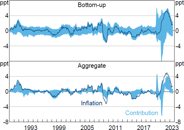
This appendix explores the robustness of the decomposition of aggregate PCE inflation in Section 4.2 to excluding the COVID-19 period from the estimation sample. The VARs are estimated using a sample that runs up to 2019:M12.^[36] The estimated sets tend to be wider than those obtained using the full estimation sample (Figure B1). For the decomposition based on aggregate data, these wider sets reflect that the estimated value of $\rho$ is substantially smaller (0.04) than in the full sample (0.18). It remains the case that the sets from the bottom-up decomposition are substantially wider than the sets obtained when using the aggregate data.

Footnote

Unlike the exercise in Section 4.2 based on the full sample of data, all category-level VARs are stable. There is consequently a (small) difference in coverage of the expenditure basket between Figures 8 and B1. [36]