RDP 2024-05: Sign Restrictions and Supply-demand Decompositions of Infation 4. Supply-demand Decompositions of US Inflation

This section builds on the insights above – in terms of using the sign restrictions to set identify the contributions of supply and demand shocks – to decompose US inflation into its drivers. I conduct two exercises that relate to existing decompositions of US inflation. The first approach is based on aggregate data and relates closely to a decomposition in Chang et al (2023), as well as possessing similarities to decompositions in Bergholt et al (2023) and Giannone and Primiceri (2024). The second approach builds a bottom-up decomposition of aggregate PCE inflation using disaggregated data on different expenditure categories, and relates to the influential decomposition proposed in Shapiro (2022).

4.1 An aggregate decomposition

Using a two-variable SVAR identified via sign restrictions, Chang et al (2023) decompose inflation and real GDP growth in the United States into contributions from shocks to aggregate supply and demand. They present historical decompositions based on a single model chosen from the set of models that are consistent with the sign restrictions using the ‘median target’ criterion from Fry and Pagan (2011). In contrast, I characterise sets of decompositions that are consistent with the identifying restrictions.

The model's endogenous variables are $y_t={\left({\pi }_t,g_t\right)}^{\prime }$, where ${\pi }_t$ is quarterly growth in the GDP deflator and g_t is quarterly growth in real GDP.^[17] Quarterly growth rates are approximated by log differences. The model includes a constant and eight lags of the endogenous variables and is estimated using data from 1989:Q1 to 2023:Q2.^[18] I estimate the reduced-form parameters via ordinary least squares (OLS) and compute the sets of decompositions conditional on these estimates.^[19]

As above, the identifying restrictions are that aggregate supply shocks move inflation and output in opposite directions and aggregate demand shocks move them in the same direction, which is equivalent to assuming the aggregate supply curve is upward sloping and the aggregate demand curve is downward sloping. Chang et al (2023) restrict the impulse responses on impact and in the period after the shocks. To avoid making assumptions about the persistence of the effects of shocks, I impose the restrictions only on impact.

Consistent with Chang et al (2023), I estimate the contributions of both current and past supply shocks to the realisation of inflation. In the notation of Section 2.2, this means that the historical decomposition of interest is H_1,t. I present decompositions of both quarterly and year-ended inflation.^[20] As discussed above, it is not possible to allocate the entirety of inflation to either supply or demand shocks, because part of inflation is explained by the constant and initial conditions. For ease of presentation, Figure 3 – which presents the estimated sets of historical decompositions – plots only the part of inflation that can be explained by shocks occurring within the sample; that is, after removing the deterministic component. On average, deterministic terms contributed about 0.5 percentage points to quarterly inflation and 2 percentage points to year-ended inflation.

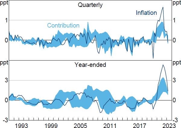
Note: Inflation is (quarterly or year-ended) growth in GDP deflator after removing contributions from constant and initial conditions.

Sources: Author's calculations; Federal Reserve Bank of St. Louis.

The correlation in the one-step-ahead forecast errors for ${\pi }_t$ and g_t is 0.47. The observed forecast errors can therefore be interpreted as roughly tracing out an upward-sloping (short-run) aggregate supply curve, but we learn nothing about the slope of the (short-run) aggregate demand curve. Although the set of historical decompositions tends to be wide, it still appears to deliver useful inferences about the drivers of inflation in some periods. For example, when year-ended inflation peaked in 2022:Q2 at 7.4 per cent, supply shocks are estimated to have contributed between 1.3 and 3.4 percentage points (deterministic terms contributed about 2.1 percentage points to year-ended inflation in this period). The estimates therefore suggest that supply shocks made a substantial contribution to the increase in inflation in this episode, though the estimates do not allow us to unambiguously conclude whether the increase was mostly driven by supply or demand shocks.

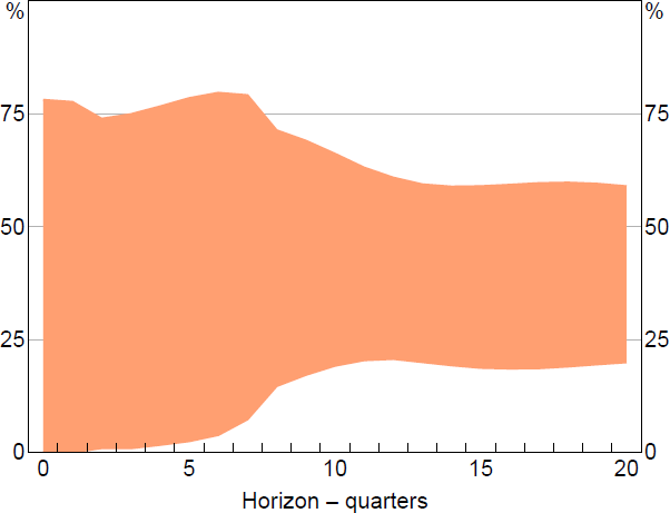
The moderate degree of correlation between the one-step-ahead forecast errors means that the identified set for the FEVD is fairly wide (Figure 4). Aggregate supply shocks are estimated to account for between zero and 78 per cent of the variance of one-step-ahead forecast errors, and between 20 and 60 per cent of the variance of forecast errors at the five-year horizon. The sign restrictions therefore do not shine much light on the drivers of aggregate inflation at short horizons, though they suggest that supply shocks make a nontrivial contribution at longer horizons.

4.1.1 Robustness

The VAR described above is estimated over a sample period that includes the COVID-19 pandemic, which is consistent with the exercise in Chang et al (2023). One may worry that the large swings in economic activity that occurred during the pandemic may unduly affect the estimates of $\varphi$ and thus the sets of decompositions generated by the sign restrictions. This section explores the robustness of the results presented above to excluding the data from this episode from the estimation sample. To do this, I omit the data from 2020:Q1 onwards.^[21] The data from 2020:Q1 to 2023:Q2 are subsequently used to construct the reduced-form VAR innovations and historical decompositions during the period after the onset of the pandemic.

Re-estimating the model over this period yields an estimate for $\rho$ around 0.01, which is much smaller than the estimate obtained over the full sample (0.47). The large reduction in $\rho$ results in sets of decompositions that are substantially less informative (i.e. much wider) than those obtained over the full sample. For example, the sets of historical decompositions for year-ended inflation tend to include zero and the realisation of inflation itself (Figure 5). In 2022:Q2, supply shocks are estimated to have contributed between 0.3 and 4.4 percentage points to year-ended inflation. Identified sets for the FEVD (not plotted) are also wide, spanning from zero to (almost) one at the impact horizon and from around 15 to around 80 per cent at the five-year horizon. Overall, after excluding the pandemic from the estimation sample, the sign restrictions appear to be largely uninformative about the drivers of inflation in the GDP deflator.^[22]

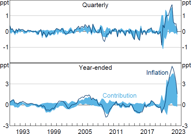
Note: Inflation is (quarterly or year-ended) growth in GDP deflator after removing contributions from constant and initial conditions.

Sources: Author's calculations; Federal Reserve Bank of St. Louis.

4.2 Disaggregated decompositions

Shapiro (2022) proposes a supply-demand decomposition of US inflation in the PCE index based on disaggregated data. The decomposition involves estimating VARs for prices and quantities consumed in different PCE expenditure groups. Given sign restrictions on the slopes of the supply and demand curves, if the price and quantity forecast errors have the same sign, a demand shock must have occurred, and the price change is classified as demand driven. If the forecast errors have opposite signs, a supply shock must have occurred, and the price change is classified as supply driven.^[23] On this basis, overall inflation is decomposed into demand- and supply-driven components.

More precisely, let the superscript k index expenditure categories. ${\pi }_t^{\left(k\right)}$ is quarterly inflation in expenditure category k and $w_t^{\left(k\right)}$ is the expenditure weight in the consumption basket. The supply-driven component of aggregate quarterly inflation is then defined as

where 1(.) is the indicator function. The demand-driven component is defined similarly.^[24]

A feature of this decomposition is that it allocates the entire price change in an expenditure category on the basis of contemporaneous demand or supply shocks even though these shocks could only contribute to the one-step-ahead forecast error (i.e. the ‘unexpected’ part of the price change). It therefore ignores the lagged effects of shocks and the contributions of deterministic terms. The decomposition may also misrepresent the direction in which shocks contribute to inflation. For example, if $u_{pt}^{\left(k\right)}<0,u_{qt}^{\left(k\right)}>0$ and ${\pi }_t^{\left(k\right)}>0$, then ${\pi }_t^{(k)}$ will contribute positively to the supply-driven component of inflation despite the model implying that a disinflationary supply shock has occurred in category k. The decomposition also allocates the entirety of the price change in a particular category to either a supply or demand shock, when it seems probable that price changes in each period are driven by a mix of supply and demand shocks.^[25]

I address these issues by directly estimating the set of historical decompositions within different expenditure categories. The concept of the historical decomposition employed is H_1,t, so the effects of all past shocks are captured. The aim of the exercise is to explore the extent to which the sign restrictions allow us to learn about the contributions of supply and demand shocks within different expenditure categories. I then use the disaggregated results to construct a bottom-up decomposition of aggregate PCE inflation and compare it against a decomposition based on the aggregate PCE data. The exercise therefore speaks to whether applying the supply-demand decomposition to disaggregated data provides useful information about the contributions of supply and demand shocks to aggregate inflation relative to applying the decomposition to the aggregate data directly.

I consider 136 expenditure categories that make up the PCE data between January 1988 and September 2023.^[26] Within expenditure category k, the endogenous variables are $y_t^{\left(k\right)}={\left({\pi }_t^{\left(k\right)},g_t^{\left(k\right)}\right)}^{\prime }$, where ${\pi }_t^{\left(k\right)}$ is monthly inflation in the PCE price index and $g_t^{\left(k\right)}$ is monthly growth in real PCE (approximated using log differences). Each VAR includes 12 lags of the variables and a constant.^[27] I estimate each VAR separately via OLS and compute sets of historical decompositions conditional on the OLS estimates of the reduced-form parameters. Though the VAR is estimated at the monthly frequency, I present historical decompositions of year-ended inflation.

As discussed in Section 3, the correlation between the forecast errors in prices and quantities is important in determining how informative the sign restrictions are about the slopes of supply and demand curves and thus about the contributions of shocks to inflation. The category with the smallest absolute correlation is ‘lubricants and fluids’ $\left(\left|\rho \right|<0.0001\right)$ and with the largest absolute correlation is ‘food produced and consumed on farms’ $\left(\rho =-0.98\right)$. Figure 6 presents the historical decompositions for these two groups.

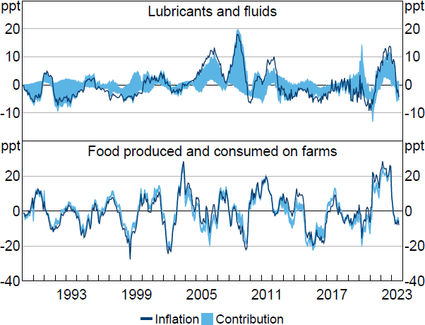
Note: Inflation is year-ended growth in price index for PCE category after removing contributions from constant and initial conditions.

Sources: Author's calculations; Bureau of Economic Analysis.

The set of historical decompositions for lubricants and fluids inflation often includes zero and the realisation of inflation itself (after removing the contribution of deterministic terms). The sets are therefore largely uninformative about whether price changes in this category are entirely driven by supply or demand shocks, which is broadly consistent with the discussion in Section 3.

In contrast, for food produced and consumed on farms, the strong negative correlation between forecast errors in prices and quantities means that the forecast errors trace out a short-run demand curve, and the contribution of supply shocks is bounded within a narrow range in most periods. To give an example, in March 2022, year-ended inflation in this expenditure category was 30.1 per cent, 28.4 percentage points of which can be explained by shocks occurring during the sample period (i.e. the contribution of deterministic components was a bit under 2 percentage points). Supply shocks are estimated to have contributed 23.9 to 25.1 percentage points to year-ended inflation in this period.

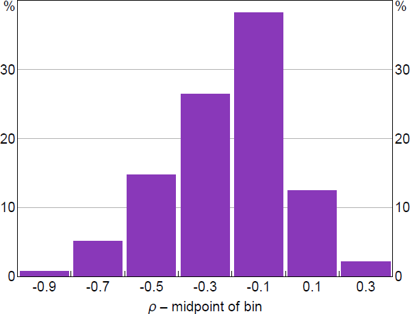
The correlation between forecasts errors tends to be reasonably weak in most other expenditure groups considered; the absolute correlations are smaller than 0.2 in about half of the categories and smaller than 0.4 in about 80 per cent of categories (Figure 7). The sign restrictions therefore tend to be fairly uninformative about the supply-demand composition of inflation outcomes within different expenditure categories.

To summarise the overall informativeness of the restrictions, I compute an expenditure-weighted average of the lower and upper bounds of the set of historical decompositions. Figure 8 presents this bottom-up decomposition of aggregate PCE inflation alongside a decomposition constructed using the aggregate PCE data directly.^[28] Separately decomposing PCE inflation in disaggregated expenditure categories does not appear to generate more informative decompositions of aggregate PCE inflation relative to a direct decomposition based on the aggregate data. In fact, the bottom-up decomposition generates substantially wider sets than the aggregate decomposition; on average over the sample period, the width of the sets is 2.6 percentage points for the bottom-up decomposition compared with 1.1 percentage points for the aggregate decomposition.

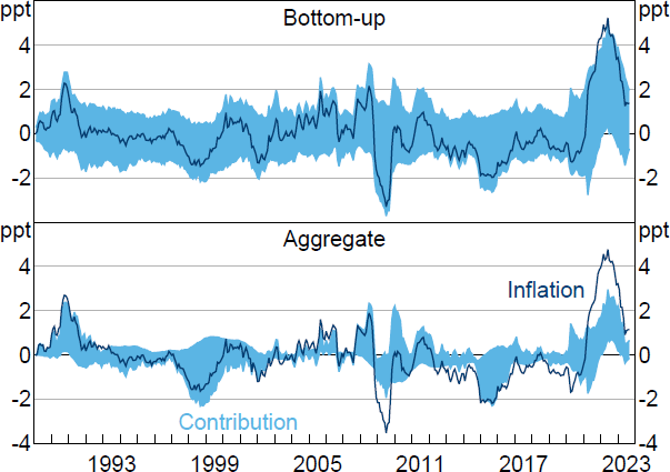
Notes: Inflation is year-ended growth in PCE price index after removing contributions from constant and initial conditions. Exercises omit two categories whose category-level VARs were unstable.

Sources: Author's calculations; Bureau of Economic Analysis.

The bottom-up decomposition clearly reveals little about the drivers of the post-pandemic surge in US inflation, admitting contributions for the supply shock ranging anywhere from around zero to the entire change (less the contribution of deterministic terms). The aggregate decomposition yields sharper conclusions; for instance, in June 2022, the aggregate decomposition suggests that supply shocks contributed between 0.7 and 3 percentage points to year-ended PCE inflation. Much like the aggregate decomposition of inflation in the GDP deflator (Section 4.1), the aggregate decomposition of PCE inflation suggests that, while supply shocks made a substantial contribution to the increase in inflation in the post-pandemic episode, the sign restrictions do not allow us to unambiguously conclude whether the increase was mostly driven by supply or demand shocks.

One reason why the bottom-up decomposition may generate less-informative decompositions of aggregate PCE inflation than using the aggregate data directly is if there is a greater degree of measurement error at finer levels of disaggregation. Intuitively, the presence of (uncorrelated) measurement error in the price and quantity data would generate one-step-ahead forecast errors that are less strongly correlated than the forecast errors that would be obtained if price and quantity were observed without error. As discussed above, weaker correlations in these forecast errors mean that the sign restrictions reveal less about the slopes of supply and demand curves and thus less about shock decompositions. Indeed, the Bureau of Economic Analysis notes that the PCE data at this level of disaggregation is of significantly lower quality than that of the higher-level categories of which they are a part, as they are more likely to be based on judgement or on less-reliable source data (Bureau of Economic Analysis 2017).^[29]

As in Section 4.1.1, re-doing this exercise with an estimation sample that excludes the COVID-19 period tends to generate wider sets, both for the bottom-up and aggregate decompositions. However, it remains the case that the bottom-up decomposition yields much wider sets than the decomposition estimated using the aggregate data directly; see Appendix B.