RDP 2025-01: Are Investment Tax Breaks Effective? Australian Evidence 6. Results
February 2025
- Download the Paper 1.89MB
6.1 Macro stabilisation policies
First, focusing on the graphical evidence for the DD approach (Figure 1), we see clear evidence of an effect for the GFC policies: investment for both groups followed a similar pattern, before diverging in the second half of 2009 when the differential tax incentive was in place (dark shading). This was particularly evident at the intensive margin.
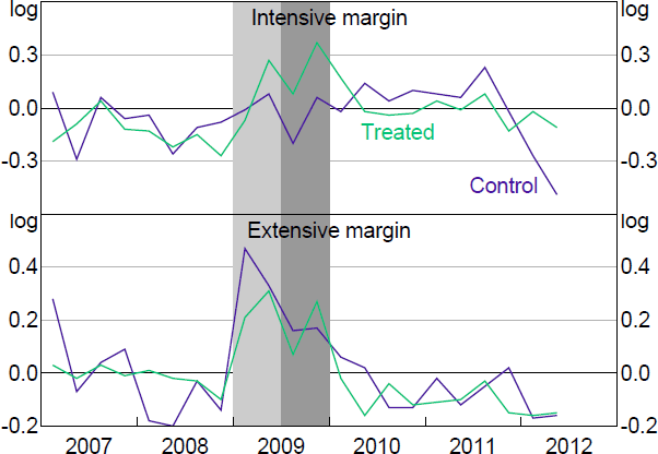
Notes: Controls for employment size, turnover decile, industry division time trends and seasonal size dummies. Light shading indicates period where treated and control firms received similar investment tax break. Dark shading indicates period with different tax breaks, which is the treatment period for regressions.
Sources: ABS; Authors' calculations.
In contrast, focusing on the COVID-19 policies (Figure 2), we can see that over this period all firm size groupings follow a broadly similar investment path. Given the overlapping nature of these policies we visualise them differently to the other DD results. We show investment for each group, where the shaded colour corresponds to the largest firm now eligible for a tax concession. If the policies were affecting investment, we would expect to see each line pick up, relative to the line for the next size group, when we enter the relevant shaded period. However, there is no evidence of an increase in investment as each group becomes eligible for the incentive, suggesting little evidence of an effect from the policy. Instead, all lines follow fairly similar paths.
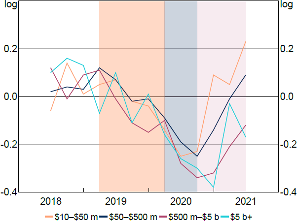
Notes: Size based on income in 2018/19. Controls for employment size, turnover decile, industry division time trends and seasonal size dummies. Shaded region indicates largest firms that were eligible for investment incentives.
Sources: ABS; Authors' calculations.
These findings are borne out in the regression analysis (Table 5). As with Rodgers and Hambur (2018), the GFC tax incentive seems to have successfully raised investment on the intensive margin, with treated firms spending substantially on eligible investment. The effects are also larger for unincorporated businesses, consistent with previous findings and the fact that the imputation system should wash out much (if not all) of the benefit for small domestically owned companies. This would also be supportive of the old view of corporate finance. Nevertheless, given there is still a response amongst companies it suggests that either the ITB is working through other channels, like easing cash flow constraints, or that there might be some heterogeneity in firm funding or ownership. For example, some firms may rely on internal funds or have overseas owners (who do not receive value from imputation credits) and so the ITB affects their cost of capital.
In contrast, we do not find statistically significant evidence that the COVID policies increased investment.[12] There is even some small evidence for a negative effect at the intensive margin for the 2020 policy but the confidence interval is wide.
| Intensive margin | Extensive margin | ||||||
|---|---|---|---|---|---|---|---|
| All firms | Companies | Unincorporated | All firms | Companies | Unincorporated | ||
| GFC 2009 | 0.456*** (0.136) |
0.414** (0.168) |
0.870*** (0.238) |
0.207* (0.113) |
0.176 (0.132) |
0.274** (0.139) |
|
| Observations | 7,226 | 4,660 | 2,520 | 46,069 | 24,758 | 21,293 | |
| COVID 2020 | −0.291* (0.150) |
0.138 (0.219) |
|||||
| Observations | 17,701 | 25,643 | |||||
| COVID 2021 | 0.404 (0.267) |
0.546 (0.449) |
|||||
| Observations | 5,040 | 6,147 | |||||
|
Notes: Mining is excluded. Regressions include controls, except for COVID 2021 intensive margin results which are estimated without controls for employment and turnover decile due to small sample sizes. ***, ** and * denote statistical significance at the 1, 5 and 10 per cent levels, respectively. Cluster robust standard errors in parentheses. |
|||||||
Turning to the RDD approach, graphically we see a clear shift down in investment after the threshold for the GFC policy (Figure 3). This is evident whether we focus on average investment within small sales buckets, or a line of best fit using a linear or local polynomial model. This is also evident in the regressions, with a large fall in investment above the threshold, suggesting the ITB raised investment for eligible firms (Table 6).[13]
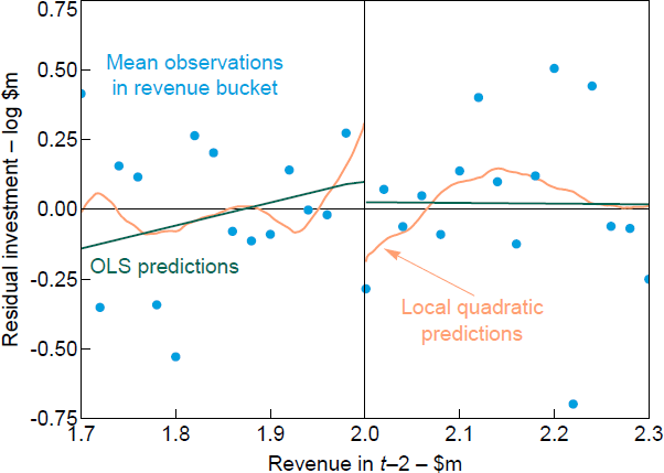
Note: Residual from a regression of log investment on industry fixed effects.
| Mar 2009 | Jun 2009 | Sep 2009 | Dec 2009 | Mar 2010 | |
|---|---|---|---|---|---|
| All firms | |||||
| Beta | −0.114 | 0.006 | −0.404** | −0.036 | −0.022 |
| Robust p-value | (0.49) | (0.79) | (0.02) | (0.82) | (0.88) |
| Bandwidth | 328,163 | 326,907 | 246,555 | 467,689 | 508,608 |
| Effective observations | 2,106 | 2,421 | 1,692 | 2,875 | 2,713 |
| Companies | |||||
| Beta | −0.127 | 0.177 | −0.154 | −0.036 | −0.155 |
| Robust p-value | (0.51) | (0.30) | (0.35) | (0.78) | (0.41) |
| Bandwidth | 374,530 | 353,778 | 313,475 | 368,003 | 560,025 |
| Effective observations | 1,332 | 1,490 | 1,173 | 1,457 | 1,685 |
| Unincorporated | |||||
| Beta | 0.005 | −0.292 | −0.570** | −0.032 | 0.187 |
| Robust p-value | (0.96) | (0.31) | (0.03) | (0.96) | (0.45) |
| Bandwidth | 315,877 | 366,361 | 275,067 | 385,634 | 466,038 |
| Effective observations | 867 | 1,084 | 813 | 1,089 | 1,081 |
|
Notes: Bolded quarters are policy periods. ***, ** and * denote statistical significance at the 1, 5 and 10 per cent levels, respectively. |
|||||
Interestingly, based on the RDD, it appears that most of the effect occurred in the first quarter of the policy (i.e. September quarter 2009), with very little evidence of an effect in the second quarter. In some sense this is surprising, as it means there was a long period between the outlay and receiving the tax benefit. The latter only happened when the company lodged its return at the end of the tax year. The finding could reflect an announcement effect. However, it could also reflect uncertainty around further changes to the policy, given the nature of what the policy would be had changed several times over the preceding year in various announcements.
The lack of a offsetting effect in the quarters following the end of the policy suggests either that the policy led to an increase in investment, rather than just a bring forward of future investment, or that the bring forward effect was quite drawn out and not readily observable. These results are consistent with Rodgers and Hambur (2018). The size of our estimates differ from theirs because we use an indicator variable to identify the 2009 GFC tax credit in contrast to their measure of the intensity of treatment. Our modelling choice is for consistency within our paper across the different policies we consider.
Unfortunately we cannot asses the COVID polices using RDD as the sample of firms close to the thresholds for the COVID-19 policies is too small to implement RDD.
The difference in the results across the GFC and COVID policies may reflect the differences in the types of economic shocks during these periods. The fact that the GFC was a financial shock that did not severely slow real activity in Australia (unemployment did not rise above 6 per cent), but may have impacted credit supply, could have meant that generous measures which increased access to funds through the tax system were more likely to be successful. In contrast, the COVID-19 shock resulted in lockdowns across Australia as well as disruptions in machinery and equipment production globally. These two factors together may have hampered the ability and incentives for business to source and install new capital purchases in order to take advantage of the investment tax breaks.
6.2 Structural small business policies
We can also compare the 2009 policy results with other small business policies to interrogate the differences in effects across the policies. For both the 2012 and 2015 policies there is very little graphical evidence of a policy effect in the DD set-up: investment for the treated and control groups follow similar paths pre treatment, with no change post treatment (see Figures 4 and 5).
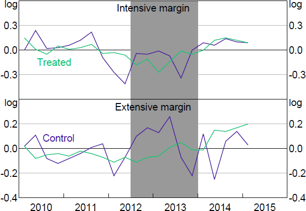
Notes: Controls for employment size, turnover decile, industry division time trends and seasonal size dummies. Shading indicates the treatment period for regressions.
Sources: ABS; Authors' calculations.
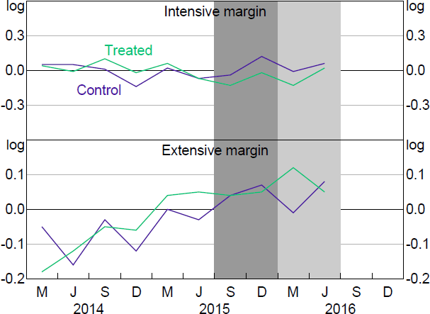
Notes: Controls for employment size, turnover decile, industry division time trends and seasonal size dummies. Dark shading indicates treatment period for DD regressions, prior to any speculation of further support. Light shading indicates period where differential investment tax break remains in place, but excluded from DD regressions.
Sources: ABS; Authors' calculations.
Consistent with this, the regression analysis suggests that the 2012 policy did not significantly raise investment (Table 7). As such we find no evidence the 2012 polices affected investment.
| Intensive margin | Extensive margin | ||||||
|---|---|---|---|---|---|---|---|
| All firms | Companies | Unincorporated | All firms | Companies | Unincorporated | ||
| GFC 2009 | 0.456*** (0.136) |
0.414** (0.168) |
0.870*** (0.238) |
0.207* (0.113) |
0.176 (0.132) |
0.274** (0.139) |
|
| Observations | 7,226 | 4,660 | 2,520 | 46,069 | 24,758 | 21,293 | |
| Small 2012 | 0.091 (0.125) |
0.031 (0.165) |
0.321 (0.200) |
0.043 (0.087) |
0.076 (0.095) |
−0.031 (0.110) |
|
| Observations | 7,253 | 4,704 | 2,521 | 49,474 | 25,920 | 23,534 | |
| Small 2015 | 0.140 (0.129) |
0.070 (0.159) |
0.440* (0.230) |
0.138 (0.100) |
0.137 (0.120) |
0.154 (0.105) |
|
| Observations | 3,911 | 2,631 | 1,270 | 24,172 | 13,298 | 10,857 | |
|
Notes: Regressions include controls. ***, ** and * denote statistical significance at the 1, 5 and 10 per cent levels, respectively. Cluster robust standard errors in parentheses. |
|||||||
There is some evidence that the 2015 policy had an effect on investment, particularly on the intensive margin for unincorporated businesses. However, it is somewhat weaker compared to the GFC policy. Furthermore, the 2015 policy may be confounded by the cuts to the corporate tax rate for small businesses that were also being implemented at the same time. As discussed below in Section 7.1, we do find some evidence these polices affected investment for companies. It is possible this could have led to some spillovers to unincorporated businesses, so the evidence of effects should be taken with some additional caution.[14],[15]
Again, the RDD results are fairly similar to the DD results. There is no evidence that the 2012 policy increased investment, even when focusing only on unincorporated businesses (Figure 6 and Table 8). The 2015 policy on the other hand did lead to some increase in investment, though only for unincorporated businesses (Figure 7 and Table 9). Again, the potential influence of the corporate tax rate cuts should be kept in mind. Moreover, the effect is evident in the March 2016 quarter, once the next set of incentives that applied to firms with up to $10 million in revenue had already been announced, which may confound the results (though the Medium 2016 policy does not seem to have had an effect).
The apparent negative impact of the policy in the June 2015 quarter, before the policy began, may be a sign that firms held off investment in anticipation of the policy. If this were the case, however, we would expect to see a strong impact of the policy in the first two quarters where it was in place (September and December 2015). However, there is no measurable impact of the policy during that period.
These lack of responses, particularly for the 2012 policy, may seem somewhat surprising in the context of the GFC results, given the targeted groups were identical. However, the 2012 changes happened in a context of heightened political uncertainty. The legislation enacting the increase from $1,000 to $5,000 was contingent on the passage of the mineral resource rent tax legislation. The further increase to $6,500 contingent on the passage of legislation related to emissions reductions. Uncertainty around these other policies, particularly the fact that the opposition party committed to unwinding these policies if it won government before the expiration of the tax break, may have led businesses to hold off on investment.
Some evidence suggests the 2015 policy had a small effect for unincorporated businesses. However, this evidence is weaker and macroeconomically less significant, given we find no aggregate economic impact. This could reflect a number of factors: heightened political uncertainty with the Australian Senate blocking government legislation and culminating in the first double dissolution election since 1987; the smaller nature of the policy; the introduction of the policy at the same time as corporate tax cuts that lowered the value of the investment tax break; and looser financial conditions, which may have meant less scope for the policy to influence companies.
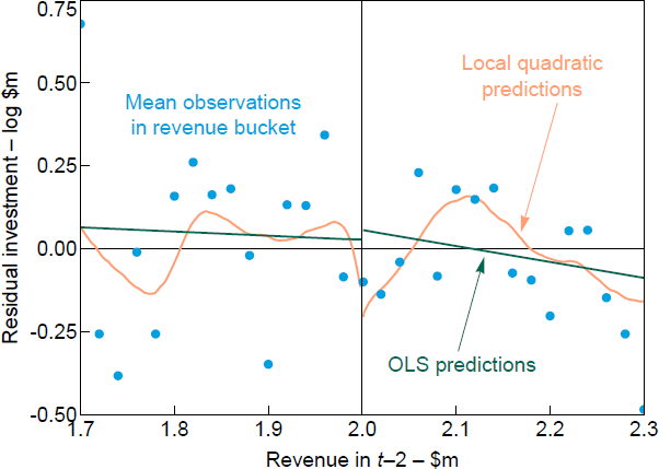
Note: Residual from a regression of log investment on industry fixed effects.
| Mar 2012 | Jun 2012 | Sep 2012 | Dec 2012 | Mar 2013 | Jun 2013 | Sep 2013 | Dec 2013 | |
|---|---|---|---|---|---|---|---|---|
| All firms | ||||||||
| Beta | −0.149 | −0.039 | −0.047 | 0.162 | 0.186 | 0.171 | −0.042 | −0.112 |
| Robust p-value | (0.53) | (0.78) | (0.85) | (0.25) | (0.26) | (0.14) | (0.93) | (0.61) |
| Bandwidth | 372,005 | 421,748 | 379,932 | 345,167 | 380,623 | 406,370 | 316,471 | 411,141 |
| Effective obs | 2,765 | 3,177 | 2,713 | 2,556 | 2,639 | 2,952 | 2,402 | 2,990 |
| Companies | ||||||||
| Beta | −0.288 | 0.091 | 0.040 | 0.187 | 0.151 | 0.527** | 0.148 | −0.173 |
| Robust p-value | (0.21) | (0.77) | (0.91) | (0.32) | (0.70) | (0.02) | (0.41) | (0.43) |
| Bandwidth | 436,224 | 390,962 | 401,357 | 456,602 | 362,765 | 323,714 | 410,413 | 539,201 |
| Effective obs | 1,664 | 1,614 | 1,470 | 1,631 | 1,312 | 1,317 | 1,531 | 1,813 |
| Unincorporated | ||||||||
| Beta | 0.298 | −0.163 | −0.149 | 0.040 | 0.203 | −0.118 | −0.121 | 0.011 |
| Robust p-value | (0.69) | (0.60) | (0.70) | (0.66) | (0.24) | (0.72) | (0.92) | (0.81) |
| Bandwidth | 381,694 | 482,329 | 360,767 | 327,458 | 434,046 | 400,103 | 290,010 | 367,851 |
| Effective obs | 1,298 | 1,557 | 1,255 | 1,170 | 1,383 | 1,371 | 1,059 | 1,344 |
|
Notes: Bolded quarters are policy periods. ***, ** and * denote statistical significance at the 1, 5 and 10 per cent levels, respectively. |
||||||||
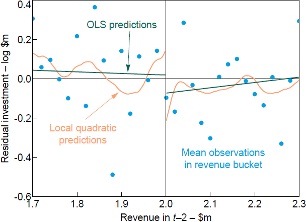
Note: Residual from a regression of log investment on industry fixed effects.
| Mar 2015 | Jun 2015 | Sep 2015 | Dec 2015 | Mar 2016 | Jun 2016 | |
|---|---|---|---|---|---|---|
| All firms | ||||||
| Beta | −0.126 | 0.226* | −0.012 | 0.055 | −0.306* | −0.279* |
| Robust p-value | (0.47) | (0.08) | (0.90) | (0.61) | (0.07) | (0.07) |
| Bandwidth | 402,386 | 344,157 | 376,464 | 407,926 | 326,053 | 368,267 |
| Effective observations | 3,234 | 3,161 | 3,129 | 3,412 | 2,915 | 3,333 |
| Companies | ||||||
| Beta | −0.258 | −0.021 | 0.180 | 0.446** | −0.136 | −0.051 |
| Robust p-value | (0.20) | (0.92) | (0.52) | (0.03) | (0.47) | (0.76) |
| Bandwidth | 334,682 | 400,725 | 385,850 | 350,061 | 451,190 | 484,585 |
| Effective observations | 1,492 | 1,875 | 1,728 | 1,688 | 1,955 | 2,154 |
| Unincorporated | ||||||
| Beta | 0.011 | 0.484** | −0.235 | −0.356 | −0.518** | −0.567** |
| Robust p-value | (0.76) | (0.01) | (0.40) | (0.10) | (0.03) | (0.01) |
| Bandwidth | 381,886 | 386,019 | 375,716 | 352,855 | 315,226 | 329,403 |
| Effective observations | 1,482 | 1,591 | 1,408 | 1,436 | 1,277 | 1,399 |
|
Notes: Bolded quarters are policy periods. ***, ** and * denote statistical significance at the 1, 5 and 10 per cent levels, respectively. |
||||||
6.3 Structural medium business policies
Focusing on the 2016 and 2019 medium business policies, which cover firms at the $10 million and $50 million thresholds, respectively, there is again little graphical evidence of an effect in the DD approach (See Figures 8 and 9). The pre-trends for the extensive margins are quite volatile suggesting that these results should be interpreted with some caution.[16]
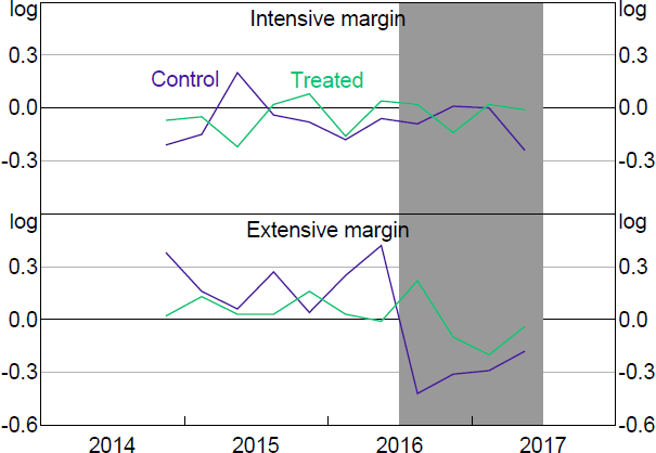
Notes: Controls for employment size, turnover decile, industry division time trends and seasonal size dummies. Shading indicates the treatment period for regressions.
Sources: ABS; Authors' calculations.
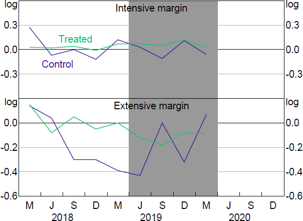
Notes: Controls for employment size, turnover decile, industry division time trends and seasonal size dummies. Shading indicates the treatment period for regressions.
Sources: ABS; Authors' calculations.
Turning to the regression results, there is some evidence of an effect at the extensive margin in the DD approach for all firms, though as noted, we should be cautious in interpreting this result (Table 10). Moreover, as discussed below, in part these results might reflect the effect of coincident corporate tax cuts (Section 7.1). Meanwhile, the 2019 policy does not appear to have increased investment.
| Intensive margin | Extensive margin | ||||||
|---|---|---|---|---|---|---|---|
| All firms | Companies | Unincorporated | All firms | Companies | Unincorporated | ||
| Medium 2016 | −0.074 (0.120) |
0.017 (0.139) |
−0.618** (0.260) |
0.295** (0.122) |
0.293** (0.142) |
0.295 (0.178) |
|
| Observations | 8,663 | 6,846 | 1,772 | 18,962 | 14,062 | 4,873 | |
| Medium 2019 | 0.034 (0.116) |
0.084 (0.125) |
−0.135 (0.253) |
−0.289 (0.203) |
−0.211 (0.200) |
−0.784** (0.336) |
|
| Observations | 7,978 | 6,732 | 1,212 | 13,646 | 11,026 | 2,593 | |
|
Notes: Regressions include controls. ***, ** and * denote statistical significance at the 1, 5 and 10 per cent levels, respectively. Cluster robust standard errors in parentheses. |
|||||||
We also show the RDD results for the 2016 policy in Table 11. There is no evidence that the policy led to increased investment. However, firms are sparser around the $10 million cut-off, as evidenced by the larger optimal bandwidth and smaller observation count. There may be too few firms to precisely estimate an RDD model for this policy.
| Mar 2016 | Jun 2016 | Sep 2016 | Dec 2016 | Mar 2017 | Jun 2017 | |
|---|---|---|---|---|---|---|
| All businesses | ||||||
| Beta | 0.099 | 0.293 | −0.247 | 0.179 | 0.140 | −0.140 |
| Robust p-value | (0.78) | (0.14) | (0.36) | (0.49) | (0.47) | (0.49) |
| Bandwidth | 2,156,505 | 2,296,991 | 1,702,082 | 2,275,956 | 1,970,100 | 1,451,920 |
| Effective observations | 1,154 | 1,224 | 1,039 | 1,218 | 1,140 | 957 |
| Companies | ||||||
| Beta | 0.144 | 0.017 | −0.272 | 0.330 | 0.401 | 0.058 |
| Robust p-value | (0.69) | (0.98) | (0.33) | (0.27) | (0.16) | (0.99) |
| Bandwidth | 2,663,093 | 2,315,771 | 1,499,775 | 2,357,502 | 1,638,978 | 1,619,548 |
| Effective observations | 874 | 852 | 670 | 874 | 712 | 695 |
| Unincorporated | ||||||
| Beta | −0.026 | 0.921** | −0.342 | −0.186 | −0.302 | −0.561 |
| Robust p-value | (0.79) | (0.03) | (0.60) | (0.75) | (0.62) | (0.19) |
| Bandwidth | 1,497,854 | 1,765,229 | 1,969,430 | 1,850,328 | 2,080,014 | 1,673,069 |
| Effective observations | 293 | 331 | 326 | 333 | 338 | 334 |
|
Notes: Bolded quarters are policy periods. ***, ** and * denote statistical significance at the 1, 5 and 10 per cent levels, respectively. |
||||||
Footnotes
Due to small sample sizes at higher turnover ranges, we do not include results by firm type for the COVID policies. [12]
For additional RDD figures see Appendix D. [13]
To the extent that some unincorporated businesses, such as trusts, are pass-through companies for corporate entities, there may also be an effect on investment for unincorporated businesses. We attempt to account for this using ABS information on business links. However, we cannot rule out the possibility that the corporate tax cuts could also affect investment of unincorporated businesses. [14]
Note that we end our DD regression in December 2015. This is because the tax cuts announced in May 2016 for firms with turnover up to $10 million may have affected the behaviour of our control group. That said, the results are broadly similar if we include the March and June quarters of 2016 in the regression. [15]
As noted above, the share of firms investing is much higher once we move to medium and larger firms. As such the extensive margin becomes a less relevant metric for these firms. [16]