RDP 33 Inflation: Prices and Earnings in Australia Appendix A: Derivation of Theoretical Model
April 1974
A firm is assumed, in the short-run, to maximise profit defined as[1] –

Subject to a production function –

Forming the Lagrangean –

The first order conditions for a maximum of (A.1) subject to (A.2) are given by the following four equations –


From (A.4) –

Substituting from (A.8) into (A.5) and (A.6) gives –


Taking the total differential of (A.7)–

| Let | yi | be the partial differential of Y(SN, ST, DL, Q) where i = 1, 2, 3 and 4 for SN, ST, DL and Q respectively, |
 |
be the part of the function Yi (SN, ST, DL, Q) which refers only to SN, ST and DL, and | |
 |
be the part of the function Yi (SN, ST, DL, Q) which refers only to Q. |
( and
and  reflect the assumption that
the marginal products are additively separable with respect to the Q component of
Yi (SN, ST, DL, Q)).
Using the above notation (A.9), (A.10) and (A.11) can be re-written as –


Now  =
=  (SN, ST, DL);
  =
=  (Q); etc.
 dXi dXi |
= | fi(SN, ST, DL) |
and  dXi dXi |
= | gi(Q) |
where Xi = SN, ST, DL and Q for i = 1, 2, 3 and 4 respectively
Hence, normalising around PN, (A.12), (A.13) and (A.14) can be re-written as –


These non-linear functions express SN, ST and DL as functions of  and Q. Therefore, it is assumed to be valid to write the following supply and demand
functions.


The partial differentials of these functions will not necessarily be constants. In most cases, depending on the specification of the production function, the partial differentials will be some function of SN, ST and DL.
The household is assumed to maximise utility –

Subject to a budget constraint –

As in the case of the firm, the first order conditions can be derived by differentiating the Lagrangean –


From (A.24) –

Substituting from (A.28) into (A.25) and (A.26) –


Dividing (A.27) through by PN gives –

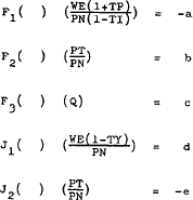
Equations (A.29), (A.30) and (A.31) express DN, DT, and SL as functions of  and
and  .
.


As in the case of the functions for SN, ST and DL the partial derivatives of these functions will not necessarily be constants. In fact J1 could change from positive to negative if the SL function was backward bending. However, this probability is assumed not to exist within the relevant range.
The three markets will be examined separately for an equilibrating mechanism. Labour market: defining excess demand for labour as –

gives –

Differentiating the excess demand function, (A.36), with respect to time gives –

For discrete time this equation can be represented as –

Where the dots denote a proportionate rate of change such that –

Setting in accordance with the signs on the partial derivatives in equations (A.20) and (A.34) –

Equation (A.38) simplifies to –

It is hypothesised that wages are set, taking account of expected changes in prices, productivity and taxes, so as to eliminate any excess demand existing at the beginning of the previous period (for fuller explanation see pp. 7–9 of the text). That is, wages are set so that –

which implies that  = 0
= 0
Where the super-script e denotes expected.
Substituting (A.40) into (A.39) and taking account of the expected changes in prices, productivity and taxes, yields the following behavioural equation for earnings –

For estimation purposes the coefficients in equation (A.41) are assumed to be constant. To simplify the notation let


where a5 and a6 are expected to be negative and the constraints implied by theory are –
| a2 + a3 | = | 1 |
| a5 + a5 | = | −1 |
| a5 | = | −a7 |
The first implies absence of money illusion while the other two arise from the fact that each of the tax variables has a relationship with excess demand for labour that is interchangeable with wages with respect to one or other of firms or households.
In order to estimate the wages equation it is necessary to eliminate two variables for which
no observable series are readily available. These are  and
and  . To remove
  the adjustment mechanism in
the tradeable goods market (detailed on p.A.10) is anticipated –

so that –

and substituted into equation (A.42). PW is world prices and ER the effective exchange rate.
There are two methods of eliminating  –
–
Method 1: As noted by Parkin [8, p.9] a relationship between award wages, prices and
productivity can be used to eliminate  –
–

Where –

Defining –

equation (A.45) can be solved for  and substituted into equation
(A.42) to give the unconstrained estimating form –

Imposing the constraints implied by theory –

Method 2:  be eliminated by making use of the aggregate price
expectations series. Solving (A.46) for
  and substituting into
equation (A.42) yields –

Imposing the constraints –

Goods market: The excess demand for non-tradeable goods is defined as –

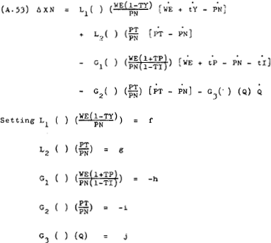
Differentiating with respect to time and converting the right-hand side variables into
proportionate rates of change (that is,  ) gives –

gives the following excess demand function –

Using the same price setting hypothesis as the labour market –

which implies that –

and allowing for expected changes in the other variables, yields the following behavioural equation for PN –

Simplifying the notation by letting b1 =  ;
b2 =
  ; etc, gives –

Where b4 and b7 are expected to be negative and the constraints on the coefficients are –
| b2 + b3 | = | 1 |
| b5 + b5 | = | b2 |
| b5 | = | −b7 |
In the tradeable goods market domestic excess demand (the difference between domestic demand and domestic supply) is –

After differentiation with respect to time this becomes –

However, while XT is generated by changes in WE, PN and so on, the adjustment mechanism is hypothesised to operate in a different manner to the previous two markets. In those markets the price of the commodity in question was assumed to respond to disequilibrium. However, in the market for tradeable goods any existing excess demand will be satisfied by imports and exports. Pricing in the tradeable goods market (as anticipated in equation (A.43) in the labour market) could therefore be expected to follow world prices adjusted for the exchange rate through international arbitrage (for a fuller explanation of this proposition see text p.10).
That is –

For discrete time period analysis the tradeable price setting process could be represented as –

As mentioned in the analysis of the labour market, series for PN and PT separately are not readily obtainable so that the estimating form for the price sector makes use of the identity (already foreshadowed by equation (A.43)) that the aggregate price level is a weighted sum of PN and PT –

Thus substituting equations (A. 57) and (A.61) for  and
and  respectively in equation (A.62) provides an unconstrained estimating form for prices –

Imposing the constraints –
