RDP 8713: Estimating the Inflationary Effects of Depreciation 2. Data

There are three key data requirements for the model used in the paper:

• a measure of world prices that is relevant to the determination of Australian import prices;
• a measure of import prices, measured in Australian currency; and
• a measure of unit labour costs.

For the first of these, an index of export prices is constructed for those countries which provide a significant proportion of Australia's non-oil imports. Weights are based on average shares in Australia's imports in the six-year period to 1985/86. The 16 included countries accounted for 83 per cent of total imports in 1985/86.^[3]

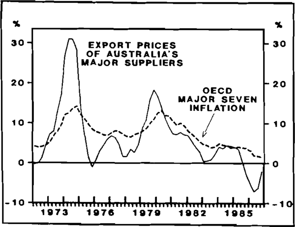
Movements in the world price variable are shown in Figure 1. Short-term movements in this index have been markedly at variance with those in more commonly-used indexes, such as the OECD area Consumer Price Index (also shown in Figure 1). While consumer price inflation in the major OECD economies slowed from mid-1985 but remained positive, this world price index actually declined between mid-1985 and end-1986. This suggests that, had there been no depreciation of the $A, prices of imports into Australia could well have fallen in 1986.^[4]

The import-price variable is the implicit price deflator for endogenous imports from the National Accounts.^[5] The deflator measures import prices on an f.o.b. basis. For the purposes of the CPI equation the deflator is multiplied by an average customs and tariff rate derived from the National Accounts, so as to give a better measure of the price that end-users of imported goods actually face.

The measure of unit labour costs is built up using data on average earnings on a National Accounts basis. This seems preferable to the survey-based measure of Average Weekly Earnings because the relevant measure according to the mark-up hypothesis should be one which regards wages as a cost rather than as an income. The National Accounts measure – wages, salaries and supplements – includes a number of “on-costs” such as superannuation contributions by employers, holiday pay and leave loadings. Furthermore, to reflect another on-cost, the earnings measure is adjusted using an average payroll-tax rate derived from the National Accounts.

The trend growth rate of productivity is subtracted from average earnings, to obtain a measure of unit labour costs. The appropriate measure of productivity is an hours-worked measure (around 0.5 per cent per quarter) rather than a per-employee measure (around 0.4 per cent per quarter). This yields a series for unit labour costs with productivity smoothed, and adjusted for payroll tax.^[6]

Footnotes

The 16 countries (in order of importance) are the United States, Japan, the United Kingdom, West Germany, New Zealand, Taiwan, Italy, Singapore, Canada, Hong Kong, France, Indonesia, Sweden, South Korea, Switzerland and Malaysia. Two countries, Saudi Arabia and Kuwait, which might have been included on the basis of their share in total imports, were excluded because the majority of those imports were petroleum-related. [3]

A similar trend emerges from OECD producer prices which also fell in this period, though not to the extent of the export price variable. Preliminary regressions using a producer price variable show very similar resuts to the preferred import price equation presented below. Both these variables provide a considerably superior explanation to a CPI variable. [4]

Endogenous imports are defined as all imported goods excluding petroleum, civil aircraft and certain large items of government expenditure, largely defence equipment. Unlike the Import Price Index (also published by the ABS), the implicit price deflator will not provide a measure of the pure price change and can be clouded by compositional change. The choice of this measure was based on the longer run of data that was available, and the fact that the import price index is a major input into the estimation of the implicit price deflator in all but the most recent quarter. Data for this and all other National Accounts variables are taken from the March 1987 Quarterly Estimates. [5]

Alternative regressions were conducted using measures of changes in actual productivity rather than the trend change in productivity. The problem with using changes in actual productivity is the amount of “noise” introduced from quarter-to-quarter movements in non-farm GDP. Even when this was smoothed somewhat, the measure gave considerably worse results in terms of goodness-of-fit. In terms of the best result appears to come from the assumption that productivity changes occur uniformly over time. [6]