RDP 8909: Optimal Wage Indexation, Monetary Policy and the Exchange Rate Regime 4. Estimation

The empirical question of interest is how close θ was to Θ over the sample period. The hypothesis θ = Θ can be tested since the parameters and variances in the model are recoverable from the data. To estimate the model equations (5) and (7) are combined to obtain an aggregate demand equation:

Two restrictions are implied from this equation:

1. π₂ = π₃;
2. π₁ + π₂ + π₄ = 0.

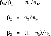
The structural parameters β₁, β₂, β₃, β₄ can be recovered from the quasi-reduced form parameters π_i as follows:

Only three parameters are estimated (π₁,π₂,π₅) but there are four structural parameters of interest (β₁,β₂,β₃,β₄). Obviously one of the structural parameters cannot be identified, and must therefore be imposed. It is convenient to choose β₁ for this purpose, and its value is set at unity. This normalization only affects the interpretation of β₄, which is now appropriately viewed as the relative interest elasticity in the model. Fortunately, the question at hand is unaffected by this normalization. Inspection of (15) reveals that the value of Θ is invariant to the value of β₁ (as is the variance of Θ).

The other equations to be estimated are for the price, wage and money supply innovations. The aggregate supply equation (3) is inverted to derive a price equation:

where γ = 1/ε and u_p = −((1+ε)/ε)u.

The wage and money supply equations are simply (4) and (6), reproduced below:

The model is estimated by a two-step procedure. First, the innovations are obtained by estimating a seven equation vector autoregression for p, y, w, m, e, g and pf.^[12] The data are quarterly, and are estimated in log difference form, with four lags allowed for each variable.^[13] The estimation period is 1973(1) to 1988(4). To conserve scarce degrees of freedom, a mixed estimation method is implemented which imposes Bayesian priors on the weights given to each variable in each regression, relatively greater weight being given to the own lags in each equation. The VAR residuals, which by construction are uncorrelated to the information set used in the first stage estimation, are the innovations to be used in the estimation of the structural model.

Since the structural model contains no exogenous variables, identification by the conventional method of zero restrictions is obviously not possible in this case. Identification is achieved instead by covariance restrictions; specifically, the structural shocks are assumed to be mutually orthogonal.^[14] An n equation system has n(n+1)/2 covariances, which is the maximum number of parameters that can be estimated, including the variances of the structural shocks. As only thirteen parameters in this seven equation system are estimated, the model is over-identified, which permits tests of the identifying restrictions. The results of these tests are reported in Appendix 2.

The model is estimated by Sargan's (1958) Generalised Instrumental Variables Estimator, a procedure which makes use of all the available instruments.^[15] Valid instruments are generated by the identification restrictions. These are firstly the e, g and pf innovations. In addition, the covariance restrictions imply that the residuals from the estimation of any structural equation can be used as instruments in the estimation of any subsequent equation.

Consistent estimates of , and are the variances of the VAR residuals from the exchange rate, government expenditure and foreign price equations, respectively. Estimates of and are the variances of the residuals in the structural equations for wages and the money supply. Estimates of and are given by

Footnotes

See Appendix 1 for data definitions and sources [12]

The VAR estimates are of no intrinsic interest and so are not reported in this paper. They are available on request from the author [13]

See Hausman and Taylor (1983) and Hausman, Newey and Taylor (1987) for comprehensive treatments of the issues pertaining to the identification and estimation of simultaneous equations models with covariance restrictions [14]

This estimator is computationally equivalent to Hansen's (1982) Generalized Method of Moments Estimator when the structural disturbances are serially uncorrelated and homoscedastic [15]