RDP 8909: Optimal Wage Indexation, Monetary Policy and the Exchange Rate Regime 2. The Model
December 1989
- Download the Paper 753KB
The model is an aggregate demand/aggregate supply specification with the variables defined in terms of their innovations i.e. unexpected components.[6] Thus, for instance, the innovations to wages are indexed to the innovations to prices. This formulation is consistent with an efficient wage contract, as rationally anticipated price increases ought to be incorporated in the base wage level.[7]
The production function is
where N is labour and u is a productivity shock. Differentiating with respect to N, setting the result equal to the real wage, and taking logs, yields labour demand:
Employment is assumed to be exclusively demand determined and so the aggregate supply function is found by substitution:
The wage indexation rule is
The other equations are
All variables, except the interest rates, are in natural logarithms, with time subscripts omitted. Equation (5) is an IS curve, with real demand a function of the real interest rate, the real exchange rate, real government expenditure and a stochastic shock. Equation (6) is a money supply reaction function. Innovations to the money supply depend negatively on innovations to the price level, and include a random component, δ. Equation (7) specifies the demand for money, with τ reflecting shocks to liquidity preference. Equations (8), (9) and (10) specify that innovations to the nominal exchange rate (the domestic price of foreign currency), real government expenditure and foreign prices have no structural determinants; they are simply random disturbances.[8] Equation (11) defines the real interest rate innovation to be the difference between innovations to the nominal interest rate and the expected inflation rate. All the shocks are assumed to be serially uncorrelated with a known finite variance, zero mean and zero covariance.[9]
The wage indexation rule, adopted for analytical convenience, is unorthodox in that wages are indexed to producer prices, rather than consumer prices (the usual basis for indexing arrangements). This is justified if the innovation in consumer prices equals the innovation in producer prices plus a random disturbance:
To see this, let wages be indexed to consumer prices:
which is also equation (4) above. x can be thought of as that part of wage innovations not captured by the indexing of wages to producer price innovations.
It is also apparent that this model contains no role for stabilizing fiscal policy. This does not mean that I adopt the counter-factual view that government purchases have no output effects. I do, however, assume that fiscal policy is not used to offset the effects of various shocks that hit the economy.
The link between monetary policy and the exchange rate is the parameter α, which can be interpreted as an indirect measure of the degree of exchange rate flexibility. When the nominal exchange rate is fixed, α = ∞ and the central bank loses all control over the money supply. Maximum control of the money supply occurs when the exchange rate is perfectly flexible (α = 0); in this case innovations to the money supply are zero up to the random shock δ. Observed deviations of α from zero under an ostensibly flexible exchange rate regime can be interpreted as evidence of intervention in the foreign exchange market by the central bank, motivated by a desire to achieve a particular exchange rate outcome.
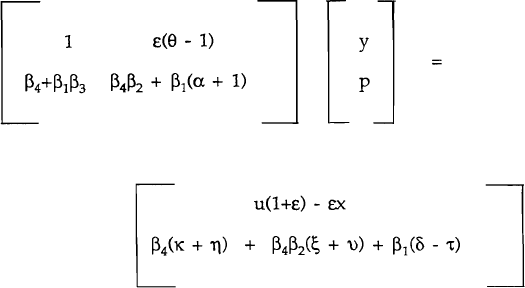
The model is solved by substituting (4) into (3), equating (6) and (7) to obtain the LM equation and then using (5) to solve for an aggregate demand equation.[10] The resulting system of equations is
The reduced form solutions are
where D = β4β2 + β1(α + 1) + ε(1 − θ)(β4+β1β3) > 0.
The comparative static properties of this model can be found in Table 1. The qualitative effects of the various shocks on output and prices are standard, and need not be elaborated in detail. It is interesting to note, however, that the effects of the demand shocks are larger the smaller is α i.e. the more flexible is the nominal exchange rate. (The corresponding effects from the supply shocks cannot be signed unambiguously.)
| SHOCK | OUTPUT RESPONSE | PRICE RESPONSE |
|---|---|---|
| u | ((1+ε)(β4β2+β1(1+α))/D > 0 | −(1+ε)(β4+β1β3)/D < 0 |
| x | −ε(β4β2+ (1+α) β1)/D < 0 | ε(β4+β1β3)/D < 0 |
| ξ,υ | β4β2(1−θ)/D ≥ 0 | β4β2/D > 0 |
| κ,s | β4ε(1−θ)/D ≥ 0 | β4/D > 0 |
| δ,−τ | β1ε(1−θ)/D ≥ 0 | β1/D > 0 |
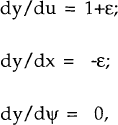
Also of interest is the special case of complete wage indexation, θ = 1. In this case
where ψ is a generic demand shock.
Under complete wage indexation, therefore, the effects of real shocks on output are independent of the degree of exchange rate flexibility (monetary policy), and demand shocks have no effect on output.
Footnotes
A model in innovation form can be derived from a general dynamic structural model. See, for example, Blanchard and Watson (1986). [6]
Implicitly, the model assumes the existence of wage contracts of length greater than one quarter. A base real wage is set at the beginning of each contract period, with provision for indexing to anticipated price increases as they occur. In addition, the contract stipulates the extent to which unanticipated price increases are passed onto wages. This is the degree of wage indexation in this model. [7]
Anticipated changes in the exchange rate are determined by monetary policy; only the innovations are assumed to be random. This specification is therefore compatible with any exchange rate regime. [8]
The assumption of zero covariance between the shocks is justified if these shocks are “primitive” i.e. without common causes. This assumption is used to identify the parameters of the model; see Section 4 below. [9]
In deriving the aggregate demand equation, the term −β1r in (5) is
replaced by −β1i and the aggregate demand shock η is replaced
by another shock s. This implies  . s is thus a linear
combination of two mean-zero random variables, and so has a mean of zero itself.
[10]


