RDP 9305: The Unemployment/Vacancy Relationship in Australia Data Appendix
June 1993
- Download the Paper 120KB
Gross Flow Data
The gross flow data are taken from the Australian Bureau of Statistics publication, The Labour Force Australia: Catalogue No. 6203.0, and is available from August 1979.
There are several sources of error in using the gross flow data:
- one-eighth of the labour force sample is replaced after each survey. Therefore the matched records from which the gross flow data are obtained can only be calculated for, at a maximum, seven eighths of the sample;
- respondents who change address in between surveys cannot be matched; and
- persons who live in non-private dwellings cannot be matched (non-private dwellings include hotels, motels, hospitals and other institutions).
The ABS estimates that those persons who can be matched in successive surveys represent about 80 per cent of all persons in the survey. About one-half of the remaining (unmatched) 20 per cent of persons in the survey are likely to have characteristics similar to those in the matched group, but the characteristics of the other half are likely to be somewhat different. It is possible to construct estimates of labour force stocks by aggregating the gross flow figures across categories in a particular period.
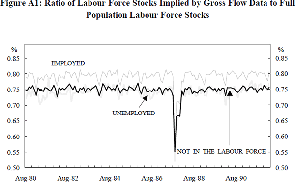
Figure A1 illustrates that the gross flow implied stocks are a relatively constant proportion of the full population labour force stocks. The large fall in 1987 is due to the survey basis being changed following the 1986 Census. It is also apparent that the implied unemployed and not-in-the-labour-force stocks for the gross flow data form a smaller proportion of the corresponding full population stocks. It is likely, therefore, that most of the error in using the gross flow data occurs in these two categories.
The series derived from the gross flow data for estimating the equilibrium UV relationship are:
- male and female inflows to unemployment;
- male and female exits from unemployment to employment;
- male and female exits from unemployment to not in the labour force;
- the total stock of unemployed; and
- the labour force stock.
The quarterly flow data are simply calculated as the sum of the monthly flows, with the quarterly stocks calculated as the averages of the monthly stocks. To be strictly compatible with the vacancy data, the stocks should be calculated at the mid-month of the quarter. However, given the error caused by the changing population basis of the gross flow data, we felt that the error would be minimised by taking the average stock over the quarter.
Gross flow estimates were not published in October 1982. The October 1982 estimates have been calculated by taking an average of the October observations in 1981 and 1983.
Vacancy Data Used in Estimating the Inflow and Outflow Equations
The vacancies data is from the Australian Bureau of Statistics publication, Job Vacancies and Overtime, Australia: Catalogue No. 6354.0, and is available quarterly from March 1977. A job vacancy is defined as a job available for immediate filling on the survey reference date, and for which recruitment action had been taken. The vacancy data relate to the middle month of each quarter.
All vacancies for wage and salary earners are represented in the survey except those:
- in the Australian permanent defence forces;
- in enterprises primarily engaged in agriculture, forestry, fishing and hunting;
- in private households employing staff;
- in overseas embassies;
- located outside Australia; and
- available only to persons already employed by the enterprise or organisation (as typically happens in the State and Federal public services).
From March quarter 1977 to December quarter 1983, the sample was selected from employers registered to pay payroll tax and government organisations. From March 1984 the sample was changed to the ABS register of businesses. This resulted in an increase in the magnitude of the vacancies reported. Vacancies under both bases were reported for December 1983. The two series were spliced together by applying the growth rates from the payroll tax series to the new series.
Each observation in the vacancy series was multiplied by 0.74, in order to make the vacancy series comparable with the unemployment series from the gross-flows data. The 0.74 figure is the average value of the ratio of the unemployment stock implied by the gross flows data to the unemployment stock from the labour force survey. The September 1987 vacancy observation was multiplied by 0.66, as during this quarter a new labour force survey was being introduced. As a result the population represented by the gross flow data constituted a smaller proportion of the total population than usual. Accordingly, the corresponding vacancy observation was scaled down.
Construction of the Index of Effective Unemployed
The index is constructed as:
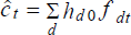
where hd0 is the exit rate at each uncompleted duration (d) in any arbitrarily selected year 0, while fdt is the proportion of unemployed at that duration in year t.
Two sources of duration data were considered, the Australian Bureau of Statistics, and the Department of Social Security. The ABS data are obtained from the labour force survey where respondents are questioned as to how long they have been unemployed. This data has proven to be unreliable as respondents tend to bunch their duration of unemployment around six months, 12 months, etc[16]. This results in a negative probability of leaving unemployment at some durations (which is impossible). The data from the Department of Social Security does not suffer from this problem as the data is derived from the Department's computer records. However the DSS data does have limitations, the most important being that it is restricted to unemployment benefit recipients[17].
One of the implications of using DSS data is that the index can only realistically be calculated for males. Generally, an unemployed married woman appears as a dependent spouse on her husband's benefit entitlement (the reverse is only rarely true), or is precluded by the income test from benefit entitlement if her husband is employed. As a result, it is considered that DSS unemployment data relating to males only provides the most accurate reflection of the labour market.
Quarterly exit rates were calculated for the durations 0 to 13 weeks, 13 to 26 weeks and so on, with the highest duration defined as over 104 weeks. These exit rates were calculated by taking the stock of unemployed at a particular duration in a quarter and comparing it with those at the following duration in the following quarter. For example, the exit rate for the 0 to 13 week duration in February (of any year) is calculated as
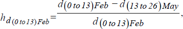
where d(0 to 13)Feb is the number of unemployed in February with duration less than 13 weeks, and similarly for d(13 to 26)May. hd(0 to13)Feb thus measures the proportion of those people who, in February, had been unemployed between 0 and 13 weeks and who left unemployment in the following 13 weeks.
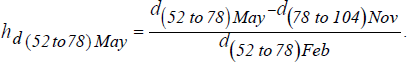
Exit rates can be similarly calculated for the 13 to 26 week duration. However, subsequent durations are only recorded over 26 week periods. Hence for these durations we first calculated six monthly exit rates; for example, the six monthly exit rate for the 52 to 78 week duration in May is:
The six monthly exit rates are converted to quarterly exit rates by using the formula:
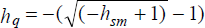
where hq and hsm are the quarterly and six-monthly exit rate rates, respectively, and where we assume that the exit rate is constant over a six month period.
The six monthly exit rate for the duration 104 weeks and over is calculated by subtracting the exits from all other durations from total terminations of unemployment benefits. Exits within the first 26 weeks are calculated by subtracting the number in the 0 to 26 week duration at the end of the 26 weeks period from the number of new grants during the preceding 26 weeks. The exit rate for the 104 week and over duration in (say) February is:
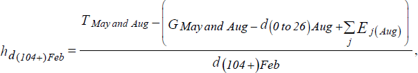
where T is terminations, G is grants and the summation is over all exits (E) from other durations.
To obtain the weights for the index, the exit rates for each duration were averaged for the period August 1985 to May 1991. This is the longest period for which exit rates can be calculated using the available data[18]. These are shown in Table A1.
| Duration (Weeks) | Males | Females |
|---|---|---|
| Just Unemployed | 0.58 | 0.61 |
| 0 to 13 | 0.43 | 0.45 |
| 13 to 26 | 0.32 | 0.35 |
| 26 to 52 | 0.27 | 0.31 |
| 52 to 78 | 0.20 | 0.24 |
| 78 to 104 | 0.19 | 0.23 |
| 104 and over | 0.15 | 0.19 |
|
Note: The exit rate for the just unemployed is shown for completeness; it is not used for computing the index. It is calculated (for May) as 2*[1−(d(0 to 13)/GrantsMay)]. We assume that the outflow rate over the first three months is constant. Therefore, by the end of a quarter, only half of the new entrants to unemployment who will exit within 13 weeks will have done so. The other half are assumed to exit in the following quarter. Source: Authors' calculations. |
||
Table A1 shows very clearly that exit rates decline as the duration of unemployment increases[19].
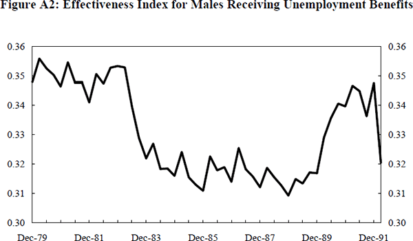
In Figure A2 we show the effectiveness index[20]. The important feature to note is that the drop in effectiveness in the early 1980s (associated with the recession of 1982–83) did not recover until the end of the decade. Though the number of long-term unemployment benefit recipients has been falling since 1987, it appears that a significant part of the improvement in the effectiveness index can be attributed to the large influx of newly unemployed from the beginning of 1990. As a result care should be taken when interpreting the large improvement in the index since 1989[21].
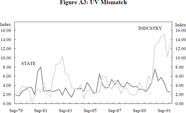
Construction of the Mismatch Indices
Due to the convexity of the Beveridge Curve, differences in the UV ratio across different groups will affect the location of the aggregate Beveridge Curve. It is therefore important to see whether any apparent movements in the aggregate curve have been caused by either regional or sectoral mismatch[22].
Following Layard et al., mismatch indices were calculated by state and sector using the formula[23].
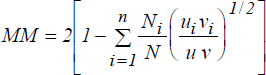
where, in category i, Ni is employment, ui is the unemployment rate and vi is the vacancy rate. A value of zero for the index indicates no mismatch.
The mismatch by state index was calculated simply by using published ABS data on vacancies and unemployment by state (including NT and ACT). Vacancies on a state by state basis are available since May 1979. As with all the ABS vacancy data used in this study, the vacancy data by state have been corrected for the change in the survey basis that occurred in November 1983. This was accomplished by applying the growth rates from the pre November 1983 payroll tax based series to the post 1983 register of businesses based vacancy series. To ensure compatibility with the vacancy data, the unemployment data are taken from the mid-month of each quarter.
Construction of the mismatch by industry index was restricted because vacancy data are available for only four sectors: manufacturing (which averaged 22 per cent of all vacancies in the sample period), wholesale and retail trade (23 per cent), public administration, defence and community services (28 per cent), and other (27 per cent)[24].
The two mismatch indices are shown in Figure A3. There appears to be slight upward trend in mismatch by both industry and state; however, the industry mismatch index is dominated by the recessions of 1982–83 and 1990–91, when it increased by about 400 per cent. The reason for this is that the job losses in these recessions were heavily concentrated in one sector – manufacturing. In the case of 1982–83, the unemployed manufacturing workers eventually left that sector, either by finding employment elsewhere, or by leaving the workforce, and those that remained unemployed for over two years were no longer classified as in the manufacturing sector. The industry mismatch index thus returned to its trend after about two years.
Construction of the Replacement Ratio
The replacement ratio is a measure of the opportunity cost of remaining unemployed. It is calculated as:

where Bt is the average entitlement to unemployment benefits, and Et is after-tax average weekly earnings. We calculated two replacement ratios, one for single adult males starting in March 1965, and one for all beneficiaries starting in September 1975.
For single adult males, Bt is simply the rate of benefit payable to a single person with no dependents. For all beneficiaries, Bt is calculated as a weighted average of all categories of all unemployment benefit recipients. The weights are the proportion of beneficiaries receiving a particular category of unemployment benefit. These categories are described in Table A2.
| Category | Comment |
|---|---|
| Under 18, Single |
From November 1984 to November 1985, a higher tax rate was paid if the person had been in receipt of benefit for more than six months. From January 1988 the under 18 years category has been named ‘Job Search Allowance’. JSA has two rates of payment subject to a parental income and assets test. |
| 18 to 20, Single | From June 1973 to November 1985, beneficiaries in this age bracket were paid the same rate of benefit as those 21 years and older. Since then they have been paid a lower rate. In September 1990 the ‘at home’ rate was introduced. The 18 to 20 year old rate continued to be paid to those who do not live with a parent. |
| 21 and over, Single | |
| Single with Children | From November 1978 a higher rate was paid to single beneficiaries with children. |
| Married Rate | |
| Additional Benefit for Children |
From December 1987 three rates of additional benefit became available. These are: (in descending payment value) children 13 to 15 years, children under 13 years, and dependent student 16 to 24 years. An average of the three rates was used in calculating the ratio. |
Et proved simpler to construct. Average weekly earnings data for males and females were obtained from the Australian Bureau of Statistics (Catalogue nos. 6350.0 and 6302.0). The series have a break at August 1981 when the data changed from being collected from payroll tax records to a survey based on the ABS register of businesses.
After-tax average weekly earnings were calculated for males back to March 1965, and for females back to September 1969. For the adult single male replacement ratio, Et is just the after tax male average weekly earnings series. For the ratio representing all beneficiaries, Et is the weighted average of male and female after tax earnings. The weights are the annual proportions of unemployment benefit recipients by sex.
One limitation of using after tax average weekly earnings to construct the replacement ratio is that it implies that the average wage is received for the entire financial year. However, a person who is unemployed part of the financial year will pay less tax than a person receiving average wages for the whole year. As a result, the measured replacement ratio will be biased towards lowering the opportunity cost of unemployment.
The replacement ratios for adult males and all beneficiaries are plotted in Figure A4. The adult male ratio increased sharply in the early 1970s (just prior to the deterioration in the labour market late in 1974) from around 15 per cent of AWE to around 25 per cent. It continued to rise until around March 1977, when it peaked at around 35 per cent of AWE. It then fell until about March 1983, and has since risen slightly.
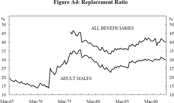
The ratio for all recipients has followed the same pattern as the male ratio, but at a higher level, reflecting the fact that unemployment benefits received by women are the same as those received by men (in the same category), but wages earned by women are on average less than those received by men.
The information on the maximum rates of unemployment benefit payable, and on changes in entitlement were obtained from the following Department of Social Security (DSS) publications: The Guide to the Administration of the Act, and Developments in Social Security: A Compendium of Legislative Changes Since 1908.
The categories of benefit entitlement were weighted by the proportion of beneficiaries receiving a particular entitlement. Annual weights were calculated from 1975 based on information in the following DSS publications: Ten Year Statistical Summary, Quarterly Survey of Unemployment Benefit Recipients, and Survey of Job Search and Newstart Allowance Recipients.
Data on an annual basis were not available for recipients in the category, ‘single with children’. However, quarterly data from February 1984 were available for this category, which had a virtually constant share at 1 per cent over this period. Hence this category received a weight of 0.01. Annual data were also not available for the average number of children for recipients in the ‘married’ category, but again these data were available quarterly from February 1984. The average number of children for the ‘married’ category over this period was 1.7, and for the ‘single with children’ category was 1.5.
Footnotes
Akerlof and Yellen (1985) call upon psychological theory to explain respondent error.
They identify three sources of error of recall of unemployment duration:
• the loss of memory of unemployment spells;
• incorrect estimation of the duration of a remembered unemployment
spell; and
• the incorrect dating of a remembered spell and the linking together
of separate spells of unemployment.
[16]
Junankar and Kapuscinski (1990) provide a detailed comparison of the DSS and the
ABS unemployment series. In particular, they list the following reasons for
the ABS and the DSS series to differ:
• recall error in ABS;
• respondent error in ABS;
• people claiming unemployment benefits when not eligible;
• people not claiming benefit when eligible, eg. because of the
fear of being ‘stigmatised’ as welfare recipients, or if the
perceived ‘costs’ of collecting unemployment benefits exceed
the benefits;
• people who are not eligible for benefits (due to the income test),
but are unemployed; and
• sampling error in the ABS series.
[17]
The average exit rate was barely changed when calculated over a longer period for those durations where longer run data are available. [18]
In interpreting our index as measuring search effectiveness of the unemployed, we
are implicitly assuming that all exits from unemployment are to employment,
but clearly this is not the case as it is quite likely that, as duration
increases, the probability of exiting unemployment by leaving the labour
force will increase. Fahrer and Heath (1992) show that this is especially
true for women which may explain why the female exit rate, at all durations,
is higher than the corresponding male exit rate. Thus our
 is probably measured with some
error as it includes the effects of both types of exit on unemployment duration.
However, we do make the important distinction between each type of exit when
estimating the equilibrium Beveridge Curve.
[19]
is probably measured with some
error as it includes the effects of both types of exit on unemployment duration.
However, we do make the important distinction between each type of exit when
estimating the equilibrium Beveridge Curve.
[19]
The spikes in the figure reflect seasonality. [20]
The absence of a large improvement in the index coinciding with the recession of 1982–83 is due to the relatively low proportion of long-term benefit recipients at that time (compared with the mid 1980s). As a result the influx of newly unemployed did not have such a dramatic effect of the index. [21]
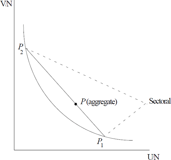
If U/N and V/N are the same across different groups then
the aggregate UV curve will be identical to that shown in the figure. But
if group one was at P1 and group two at P2 the aggregate
UV curve would be at P. Because of the convexity of the relationship UV
mismatch will always move the curve outwards.
See Layard et al. (1991) pp 325–328 for a derivation of this index. [23]
‘Other’ comprises electricity, gas and water; transport and storage; communication; mining; construction; finance, property and business services; and recreation, personal and other services. [24]