RDP 9305: The Unemployment/Vacancy Relationship in Australia 3. Estimation of Simple Beveridge Curves
June 1993
- Download the Paper 120KB
In this section we estimate some simple Beveridge Curves, i.e. regress the unemployment rate (or transformations of it) on the vacancy rate. Our purpose here is destructive rather than constructive. We aim to show that such simple methods cannot satisfactorily explain the relationship between these two variables and thus more sophisticated methods, such as we employ in Section 4, are necessary to do so.
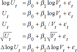
Our starting point is Harper (1980), who estimates the following functional forms for the BC over the period 1952 to 1978[2]:
where Ut is the unemployment rate, Vt is the vacancy rate (the ratio of vacancies to the labour force) and εt is a random disturbance.
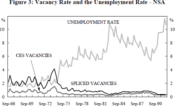
We estimate each of these relationships using seasonally unadjusted quarterly data over the period September 1966 to June 1992. This is the longest period for which consistent labour force data are available. The unemployment data refer to total unemployed (i.e. both full-time and part-time) and are measured at the mid-month of each quarter. Two vacancy series are used, ‘spliced’ vacancies and ‘CES’ vacancies.
The spliced vacancy series is similar to the NIF vacancies used by Chapman (1990), the primary difference being that the NIF series is seasonally adjusted. The series is created by splicing the ABS vacancy series onto the CES vacancy series[3]. For example, every June quarter CES unfilled vacancy observation is multiplied by the ratio of ABS vacancies to CES vacancies in June 1980. Similarly, every September CES vacancy figure is multiplied by the ratio of ABS to CES vacancies in September 1979, and so on.
The ABS vacancy series has a break in the December quarter 1983 when the sample basis moved from payroll tax records to a survey of employers. This resulted in an increase in the magnitude of the vacancies reported. Vacancies under both bases were reported in December 1983, and we have increased the payroll tax series proportionately.

The ‘CES’ vacancy series uses CES unfilled vacancy data from the September quarter of 1966 to the June quarter of 1992. Unfortunately the CES did not report unfilled vacancies during the period December 1980 to March 1983. The missing observations are constructed by applying the percentage changes from the ABS series.
The CES vacancy data are inferior to the ABS data in several respects: during periods of labour market slack, the fall in vacancies will be exaggerated as firms will not find it necessary to contact job seekers through the CES; the number of vacancies reported will vary as CES offices open and close; vacancies may be reported as unfilled when in fact they have been filled, but not by CES registered applicants; as notification of vacancies to the CES is voluntary, many vacancies are not registered; and the number of vacancies reported to the CES may vary as a result of changes in government or CES administrative policy.
The estimation results are presented in Tables 1(a) and 1(b). While the estimated coefficients on the vacancy variables have the correct sign and the standard errors of these estimates are small, the very low values of the Durbin Watson statistics indicate that the specifications are seriously in error. In all likelihood, the dynamics in these models (there aren't any) have been mis-specified. As a first step towards correcting this problem, we estimated an autoregressive distributed lag model, with initially four lags of the dependent variable (log Ut) and each exogenous regressor in the specification.
| logUt | Ut |  |
ΔlogUt | Constant | logVt |  |
 |
ΔlogVt |  |
DW |
|---|---|---|---|---|---|---|---|---|---|---|
| * |
0.67 (6.4) |
−1.03 (−12.4) |
0.61 |
0.2 |
||||||
| * |
1.80 (3.7) |
−4.3 (−11.3) |
0.56 |
0.2 |
||||||
| * |
1.83 (2.4) |
94.9 (5.9) |
0.25 |
0.1 |
||||||
| * |
3.9 (14.5) |
−0.30 (−6.6) |
0.30 |
0.1 |
||||||
| * |
−0.14 (−6.7) |
−0.10 (−1.9) |
0.65 |
1.8 |
| logUt | Ut |  |
ΔlogUt | Constant | logVt |  |
 |
ΔlogVt |  |
DW |
|---|---|---|---|---|---|---|---|---|---|---|
| * |
1.48 (29.9) |
−0.90 (−23.3) |
0.85 |
0.4 | ||||||
| * |
5.17 (26.3) |
−4.0 (−25.8) |
0.87 |
0.5 |
||||||
| * |
0.55 (1.3) |
272.1 (16.4) |
0.73 |
0.3 |
||||||
| * |
4.2 (32.1) |
−0.30 (−6.6) |
0.75 |
0.4 |
||||||
| * |
−0.15 (−7.3) |
−0.17 (−2.9) |
0.66 |
1.9 |
||||||
| Note: Asterisks indicate the dependent variable for the particular regression. All the regressions were estimated using OLS, and the figures in parentheses are the t statistics. Ut and Vt refer to the unemployment rate and the vacancy rate respectively. |
||||||||||
In addition to lags of log Vt, the regressors include the ratio of unemployment benefits to average earnings (the ‘replacement ratio’), the gap between actual and potential GDP, and a time trend[4]. The replacement ratio is included as a regressor since it measures the opportunity cost of unemployment i.e., as the replacement ratio increases, the incentive for the unemployed to search for employment falls, and so the Beveridge Curve shifts outwards, and for each vacancy rate, the unemployment rate increases. The GDP gap is included to account for the cyclical movements in the unemployment-vacancy relationship. Dummy variables were included to test for breaks in the relationship in September 1974 and September 1982.
The estimation was conducted sequentially by Ordinary Least Squares. A series of F-tests were carried out to identify and eliminate insignificant lags, resulting in the following specifications:
Using spliced vacancies:
Using CES vacancies:
where P(LM.) is the significance level at which a Lagrange Multiplier test for first or fourth order autocorrelation can be rejected.
As can be seen from equations (1) and (2), the results for both vacancy series are virtually identical. Lagged, but not contemporaneous, vacancies are significant, as is the first lag of log unemployment and the log GDP gap. The lagged, two quarter, change in the log of the replacement ratio is also significant, as is the deterministic time trend. There is clear evidence of a structural break in the third quarter of 1974, but not in 1982. The LM tests reject first-order serial correlation (at conventional significance levels), but there is some evidence of fourth order serial correlation.
The autoregressive distributed lag model is clearly an improvement on the static Harper specifications, but is still unsatisfactory in that it does not distinguish short-run movements in the Beveridge Curve, due to the business cycle, from changes in the equilibrium relationship between unemployment and vacancies. We address this issue in the following section.
Footnotes
In making this point, we are not criticising Harper's study, which is in fact the most complete examination of the Australian unemployment-vacancy relationship to date of which we are aware. Harper could not have used gross flow data to estimate equilibrium Beveridge Curves, as we do in Section 4, since such data did not exist at the time he published his paper. [2]
From September 1966 to June 1979 the vacancies series is the Commonwealth Employment Service (CES) stock of unfilled vacancies. From September 1979, we use the ABS vacancy series. The CES vacancies are spliced on to the ABS series by taking a ratio of the two series during the overlapping period, September 1979 to June 1980. [3]
The GDP gap was calculated using the Hodrick-Prescott filter, a technique which fits a nonlinear trend through the data (Hodrick and Prescott 1981). The replacement ratio is that for single males aged over 21 with no dependants. We discuss the construction of the replacement ratio in detail in the Data Appendix. [4]


