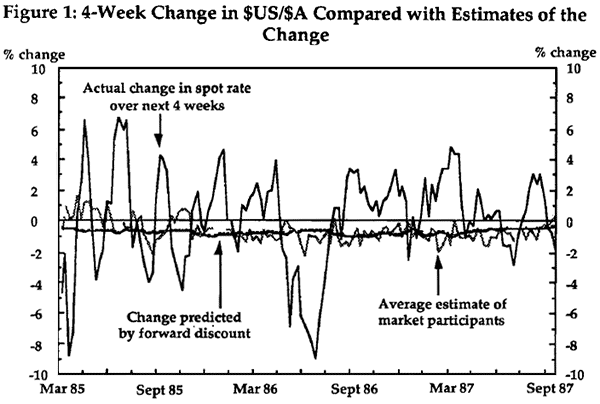
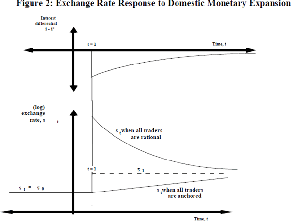
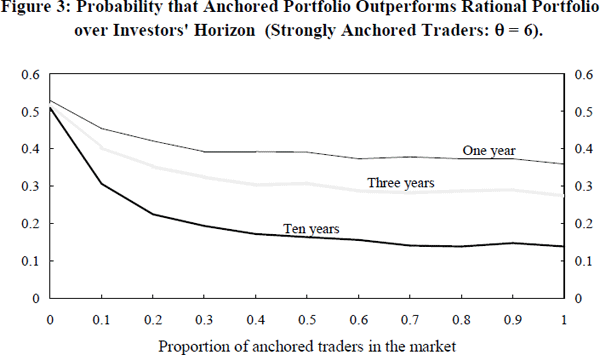
RDP 9307: Explaining Forward Discount Bias: Is it Anchoring? Tables and Figures
June 1993
- Download the Paper 119KB
| Country Pair | Mean Interest Differential (% p.a) |
Standard Deviation of Interest Differ. (% p.a) |
θ (4-week periods) |
|---|---|---|---|
| UK-US ('79–'91) | 2.9 | 2.8 | 12.3 |
| Ger-US ('79–'91) | −1.9 | 1.8 | 6.9 |
| Jap-UK ('81–'91) | −5.6 | 2.0 | 12.9 |
| Jap-Ger ('81–'91) | −0.9 | 1.9 | 26.3 |
| Jap-US ('81–'91) | −2.7 | 2.2 | 17.4 |
| θ (periods) | λ (periods) | σm (per period) | σe (per period) | β (per period) |
|---|---|---|---|---|
| 6 | 6.4 | 0.0052 | 0.031 | 0.17 (weakly anchored) 1.50 (strongly anchored) |
| 50 | 18.2 | 0.0053 | 0.031 | 0.02 (weakly anchored) 0.18 (strongly anchored) |
| θ | Investors' horizon (Years) | Markov chain para-meter | All anchored traders are weakly anchored (β = 1/θ) | All anchored traders are strongly anchored (β = 9/θ) | ||
|---|---|---|---|---|---|---|
| q |  |
 |
 |
 |
||
| 6 periods (24 weeks) |
One | 0.1 | 0.37 | 0.23 | 0.22 | −0.13 |
| 0.3 | 0.42 | 0.14 | 0.33 | −0.17 | ||
| 0.5 | 0.44 | 0.09 | 0.40 | −0.13 | ||
| 1.0 | 0.45 | 0.06 | 0.45 | 0.06 | ||
| Three | 0.1 | 0.27 | 0.45 | 0.14 | 0.11 | |
| 0.3 | 0.35 | 0.28 | 0.25 | 0.02 | ||
| 0.5 | 0.39 | 0.19 | 0.34 | 0.00 | ||
| 1.0 | 0.42 | 0.13 | 0.42 | 0.13 | ||
| Ten | 0.1 | 0.18 | 0.63 | 0.08 | 0.37 | |
| 0.3 | 0.26 | 0.46 | 0.17 | 0.24 | ||
| 0.5 | 0.31 | 0.35 | 0.25 | 0.20 | ||
| 1.0 | 0.37 | 0.23 | 0.37 | 0.23 | ||
| 50 periods (200 weeks) |
One | 0.1 | 0.51 | 0.31 | 0.34 | 0.09 |
| 0.3 | 0.48 | 0.34 | 0.41 | 0.11 | ||
| 0.5 | 0.50 | 0.31 | 0.46 | 0.18 | ||
| 1.0 | 0.50 | 0.32 | 0.50 | 0.32 | ||
| Three | 0.1 | 0.43 | 0.41 | 0.24 | 0.21 | |
| 0.3 | 0.45 | 0.39 | 0.35 | 0.19 | ||
| 0.5 | 0.48 | 0.35 | 0.41 | 0.24 | ||
| 1.0 | 0.47 | 0.36 | 0.47 | 0.36 | ||
| Ten | 0.1 | 0.31 | 0.58 | 0.13 | 0.41 | |
| 0.3 | 0.37 | 0.50 | 0.25 | 0.34 | ||
| 0.5 | 0.41 | 0.44 | 0.33 | 0.34 | ||
| 1.0 | 0.43 | 0.41 | 0.43 | 0.41 | ||
| Variables (Regression No.) |
OLS estimates (OLS std.errors) Constant Slope |
R2 | S E | D-W | ||
|---|---|---|---|---|---|---|
| st – st−1 on ft−1 – st−1 (1) |
Data | −0.016 | −4.30 | |||
| (0.006) | (1.70) | 0.041 | 0.035 | 2.19 | ||
| Model | 0.001 | −0.11 | ||||
| (0.001) | (0.46) | 0.000 | 0.032 | 2.05 | ||
| st on ft (2) | Data | −0.003 | 1.001 | |||
| (0.001) | (0.001) | 1.000 | 0.002 | 0.37 | ||
| Model | 0.000 | 1.000 | ||||
| (0.000) | (0.000) | 1.000 | 0.002 | 0.31 | ||
| st on ft−1 (3) | Data | −0.009 | 0.990 | |||
| (0.012) | (0.016) | 0.963 | 0.036 | 2.05 | ||
| Model | 0.002 | 0.998 | ||||
| (0.001) | (0.002) | 0.995 | 0.032 | 2.03 | ||
| Δst on Δft (4) | Data | 0.000 | 1.002 | |||
| (0.000) | (0.002) | 0.999 | 0.001 | 1.60 | ||
| Model | 0.000 | 1.002 | ||||
| (0.000) | (0.001) | 0.999 | 0.001 | 2.23 | ||
| Δst on Δft−1 (5) | Data | 0.002 | −0.063 | |||
| (0.003) | (0.082) | 0.004 | 0.036 | 1.96 | ||
| Model | 0.001 | −0.023 | ||||
| (0.001) | (0.022) | 0.001 | 0.032 | 2.00 | ||
| st – st−2 on ft−1 – st−2 (6) |
Data | −0.001 | 0.940 | |||
| (0.003) | (0.083) | 0.461 | 0.036 | 1.93 | ||
| Model | 0.001 | 0.977 | ||||
| (0.001) | (0.022) | 0.487 | 0.032 | 1.99 | ||
| st – st−3 on ft−1 – st−3 (7) |
Data | −0.002 | 1.054 | |||
| (0.003) | (0.061) | 0.670 | 0.036 | 2.18 | ||
| Model | 0.001 | 1.003 | ||||
| (0.001) | (0.016) | 0.661 | 0.032 | 2.04 | ||
Data are McCallum's results for $/DM, monthly 1978:1 to 1990:7. Model results are based on a 2000 period simulation assuming investors' horizon is one year, q = 0.1, θ = 6 and strongly anchored traders (β = 9/θ).


 and the coefficient
 , from the regression
Δst+1 =