RDP 9706: Is the Phillips Curve A Curve? Some Evidence and Implications for Australia 4. Empirical Results
October 1997
- Download the Paper 237KB
This section presents empirical results from the estimation of linear and non-linear Phillips curves for Australia using model-consistent estimates of the NAIRU. As described above, the NAIRU is modelled as a time-varying parameter which follows a random walk through time.
4.1 Basic Results
Results for the two models of the Phillips curve are shown in Table 1. For the results reported in this section, we measure the forward-looking component of inflation expectations by the difference between the Australian 10-year bond yield and an estimated global real interest rate (as discussed in Section 3).
| Phillips curve: | ||||||
|---|---|---|---|---|---|---|
 |
||||||
where  |
||||||
| γ | δ | LLF | σ2 | α | max[u-u*] | max[Δu*] |
| 1.25 | 0.09 | 16.27 | 0.49 | 1.17 | 6.01 | 1.46 |
| (3.08) | (2.54) | |||||
| (3.47) | (1.60) | |||||
| Phillips line: | ||||||
 |
||||||
| where |
||||||
| γ | δ | LLF | σ2 | α | max[u-u*] | max[Δu*] |
| 0.27 | 0.17 | 26.92 | 0.18 | 0 | 9.31 | 4.47 |
| (1.34) | (2.19) | |||||
| (4.26) | (2.18) | |||||
| t-statistics in parentheses: unadjusted, and Newey-West corrected | ||||||
| γ | labour-market sensitivity parameter | |||||
| δ | weight given to forward-looking component of inflation expectations | |||||
| LLF | value of the log-likelihood function | |||||
| σ2 | standard error of the equation | |||||
| α | average value of u-u* | |||||
 |
forward-looking inflation expectations based on bond yields, equal to the 10-year bond rate less the world real interest rate | |||||
The table shows estimated parameters for both the linear and non-linear models and the value of the likelihood function associated with each model. Standard errors are reported for γ and δ. Given the presence of autocorrelation, in part induced by the use of a four-quarter-ended inflation rate (rather than a quarterly inflation rate), we correct the raw standard errors using the Newey-West (1987) approach. Therefore, the first line in parentheses in the table reports the unadjusted t-statistics while the second reports the Newey-West t-statistics.
The parameter α measures the difference between our estimate of the NAIRU (u*) and the natural rate of unemployment which we proxy by the average value of unemployment over the sample.[11] We also show the maximum size of the unemployment gap over the estimation period, and the largest change in the NAIRU in any one quarter.
δ, the weight that wage and price setters place on the forward-looking component of inflation expectations, is 0.09 for the non-linear model, and 0.17 for the linear model. In each case, δ is statistically significant at the 5 per cent level, using the unadjusted standard errors, but is insignificant in the non-linear model when the standard errors are adjusted to take account of the autocorrelation. The low value of δ implies that for the most part inflation expectations are formed adaptively. The value of δ presented here is consistent with estimates of 0.15, 0.20 and 0.08 reported in Debelle and Laxton (1997) for Canada, the United Kingdom and the United States respectively.
In both models, γ has the expected sign. The value of γ in the non-linear model measures the degree of convexity in the curve. The functional form that we estimate implies that the response of inflation to a one percentage point change in the unemployment rate varies with the level of both the NAIRU and the actual unemployment rate. For example, assuming that the NAIRU is 6 per cent, a one percentage point fall in the unemployment rate from an initial value of 6 per cent leads to a rise in inflation (above expectations) of 0.22 percentage points. However, if unemployment falls a further one percentage point, inflation increases by a further 0.31 percentage points. The convexity implies that further falls in unemployment lead to even larger rises in inflation. In the linear model, a one percentage point fall in the unemployment rate always leads to a 0.27 percentage point rise in inflation, regardless of the level of unemployment or the NAIRU.
Thus, in the region of the NAIRU, the linear and non-linear models are approximately equivalent. The important distinction is when the economy is further away from equilibrium.
Convexity in the Phillips curve implies that the NAIRU will always be less than the expected value of the unemployment rate in the stochastic steady state. α depends on the amplitude of the fluctuations of unemployment around its expected value. These results suggest that for Australia over the sample period, the unemployment rate was on average 1.17 percentage points above the NAIRU. This compares to estimates of 0.86 for Canada, 0.57 for the United Kingdom and 0.33 for the United States, presented in Debelle and Laxton (1997). One explanation for the higher value for Australia might be that the size of the shocks affecting the Phillips curve equation were larger here than in other countries.
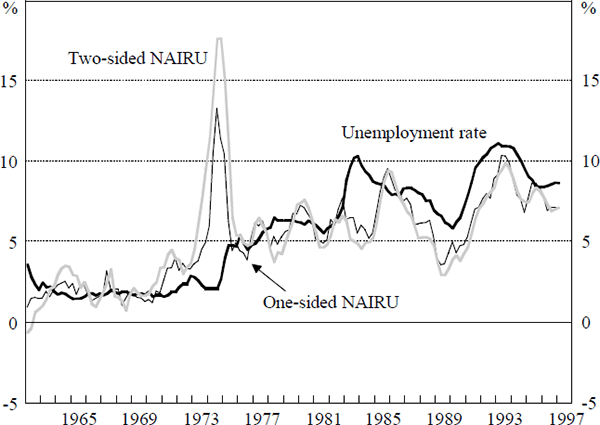
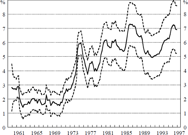
As discussed above, given the estimate of γ, we can derive time paths for the NAIRU. These are shown for the linear and non-linear model in Figures 3 and 4. For both models, both the one-sided and two-sided estimates of the NAIRU are shown (Section 3.2).
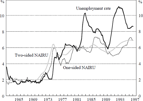
In the non-linear model, the one-sided estimate of the NAIRU remains at approximately 2 per cent through the 1960s, before rising to a level around 6 per cent around the time of the sharp increase in real wages in 1974. After falling slightly during the rest of the 1970s, the estimate again increases at the turn of the decade. Thereafter, the estimate of the NAIRU fluctuates in the range between 5 and 8 per cent. The most recent estimate of the NAIRU (1997:Q1) produced by the non-linear model is 6.9 per cent. This figure is slightly lower than the point estimates of most researchers, although inside the confidence bounds reported in Crosby and Olekalns (1996).
The two-sided estimate is clearly smoother than the one-sided estimate. When there is a difference between the two estimates, the estimated value of the NAIRU based on information available at the time has been revised in the light of later data. In periods where the two-sided NAIRU is above the one-sided NAIRU, the central bank would have run policy which in retrospect might appear too loose. For example, during the early 1970s, a policy-maker using this framework would have underestimated the level of the NAIRU in real time (using the one-sided estimates) and thus would have erred on the side of overly loose policy. Conversely, in the period 1986–1989, the real time estimate of the NAIRU lay below the smoothed estimate implying that if one used this framework, policy would have been relatively tight. However, the one-sided estimate always lies within the confidence interval of the two-sided estimate, highlighting the large degree of uncertainty associated with estimating the NAIRU.
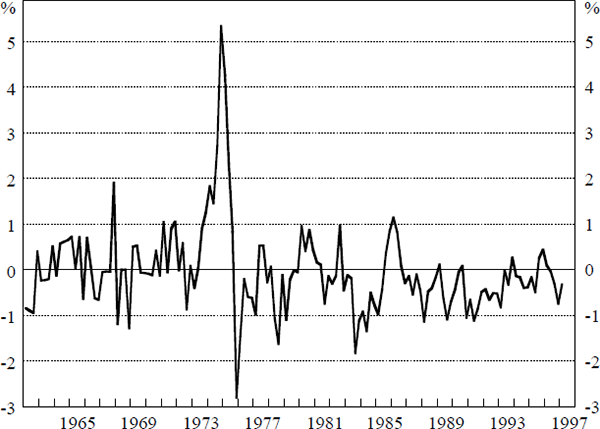
The non-linear estimates of the NAIRU suggest that the actual unemployment rate has been above the NAIRU throughout most of the 1990s. This is because inflation expectations have exceeded inflation over this period. Figure 5 plots the difference between actual inflation and the level of inflation expectations in the non-linear model.[12] In this framework, if inflation expectations were lower, then a smaller unemployment gap would be consistent with maintaining inflation at the targeted level. This demonstrates that inflation expectations have been slow to adjust downwards to the new low inflation environment. The slow adjustment of expectations increases the adjustment cost in terms of output/unemployment.
4.2 The Linear versus the Non-linear Model
The time path of the NAIRU exhibits considerably larger fluctuations in the linear model than in the non-linear case. In the linear model, the NAIRU increases rapidly from 2 per cent in 1970 to over 10 per cent in 1974, before falling back to around 5 per cent in the mid 1980s. The final point estimate of the NAIRU using this model is 7.1 per cent.
The largest quarterly movement in the NAIRU in the linear model is 4.5 per cent, compared to only 1.4 per cent for the non-linear model. The larger movements in the NAIRU, such as those in the latter part of the 1980s shown in Figure 4, are necessary for the linear model to obtain a good fit of the data. As mentioned above, the convexity in the non-linear model allows it to capture periods of a large difference between actual and expected inflation with a relatively small gap between the actual unemployment rate and the NAIRU. The linear model fits such periods by moving the NAIRU more.
Movements in the NAIRU ought to reflect the changing structural features of the labour market. Our priors would thus suggest that the series should therefore evolve slowly over time, rather than exhibiting the large quarterly fluctuations in the linear model specification. On this basis, the non-linear model represents a path for the NAIRU which is more in accordance with the way the labour market is generally thought to operate. Nevertheless, the linear model has a higher value of the log-likelihood function than the non-linear specification.
Since estimating the linear model results in unrealistically large quarterly variations in the NAIRU in order to obtain a better fit to the data, we estimate a restricted model where the signal-to-noise-ratio is adjusted to restrict the variation in the NAIRU. This restricted model considerably reduces the value of the likelihood statistic, that is the degree of fit, to 9.92 – less than the non-linear model (although the difference between the two models is not statistically significant). Thus, imposing a reasonable amount of time variation in the NAIRU on the linear model can only be achieved with a substantial loss of fit.
4.3 Alternative Estimates of Inflation Expectations
In this section we examine how the above results are affected by alternative estimates of inflation expectations. We consider three alternative processes. In the first, a richer dynamic structure is used for the formation of the backward-looking component of inflation expectations. In the second, expectations are formed entirely adaptively, and are modelled only using lags of the rate of change of the consumer price index. Thirdly, expectations are modelled using the Melbourne Institute inflation expectations series. This series, which is available from 1973 onwards, is based on survey data.
A comparison of actual underlying inflation, as well as inflation expectations based on bond yields and the Melbourne Institute survey, is presented in Figure 6.[13] For reference, we also include an expectations series derived from indexed bonds, although this time series is not long enough to include in our estimation. Two features of this figure are notable:
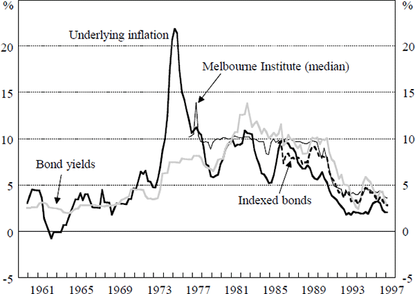
- Both the bond yields and survey measures produce estimates of inflation expectations which overstate actual inflation through most of the 1980s.
- The Melbourne Institute series tracks the bond-yield and indexed-bond measures of inflation expectations quite closely, especially since the mid 1980s.
In the first alternative specification, the model is extended to include additional lags of the inflation rate, so that the process generating inflation expectations is:

If inflation is best characterised as a unit root process, then it may be appropriate to restrict the sum of the right-hand side variables to equal one. In the estimation conducted here, this restriction is not imposed on the model.[14] Note however, that in a successful inflation-targeting regime, the inflation rate may more likely be stationary.
Summary results for including this specification for inflation expectations in the nonlinear model are presented in Table 2.
|
||||||
|---|---|---|---|---|---|---|
where  |
||||||
| γ | δ | LLF | σ2 | α | max[u-u*] | max[Δu*] |
| 0.66 | 0.12 | 32.19 | 0.30 | 2.8 | 7.9 | 1.31 |
| (1.28) | (1.92) | |||||
| (3.42) | (2.98) | |||||
| t-statistics in parentheses: unadjusted, and Newey-West corrected | ||||||
| γ | labour-market sensitivity parameter | |||||
| δ | weight given to forward-looking component of inflation expectations | |||||
| LLF | value of the log-likelihood function | |||||
| σ2 | standard error of the equation | |||||
| α | average value of u-u* | |||||
|
forward-looking inflation expectations based on bond yields, equal to the 10-year bond rate less the world real interest rate | |||||
Only the first of the four lagged inflation terms was significant at the 5 per cent level of significance. The final point estimate of the NAIRU based on this model specification is 6.5 per cent. The time path of the NAIRU is also somewhat different than in the previous case, with the main rise in the NAIRU occurring in the second half, rather than the first half, of the 1970s; followed by a further rise in the early part of the 1990s. More generally, the time path of the NAIRU, as well as its final point estimate were quite sensitive to the lag length chosen for the adaptive component of the inflation expectations variable.
The results for the other two expectations processes are presented in Tables B.1 and B.2 in Appendix B. In both cases, the NAIRU became more volatile than in the case where bond yields were used to model forward-looking expectations. This was especially so when the Melbourne Institute series for inflation expectations was used in the model.[15]
4.4 Speed Limits in the Phillips Curve Specification
To capture the possibility of ‘speed-limit’ effects, an unemployment change variable is included in the non-linear and linear Phillips curve specifications in Table 1. The specification of the non-linear model then becomes,
Such a specification is compatible with the view that rapid reductions in the unemployment rate (such as that which occurred in Australia during 1994–1995) are associated with increased inflationary pressure. Thus, χ would be expected to be negatively signed. However, χ is not significantly different from zero at the 5 per cent level of significance in either model, and actually has a positive sign (the results are in Table B.3 in Appendix B). When the models were re-estimated using data from 1980 onwards, χ had the expected sign in the non-linear model, but was still not statistically significant, while in the linear model it remained slightly positive.
4.5 Sensitivity of the NAIRU Estimates
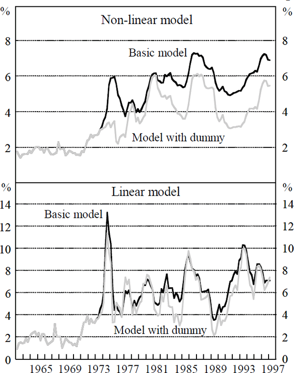
In addition to changing the specification of inflation expectations, we also included a number of dummy variables to account for various exogenous shocks to inflation over the estimation period, that ought not necessarily be reflected in movements in the NAIRU. We include a dummy variable for the period 1973:Q2 to 1975:Q2 to take account of the first OPEC oil price rise and the large wage increases in 1974. We also include dummy variables for the 1982 wage freeze, and the wage-tax tradeoffs of the late 1980s. Only the OPEC dummy variable is significant. Including the dummies results in a substantially smaller rise in the NAIRU in the mid 1970s in the non-linear model. In the linear model, the spike in the NAIRU in 1974 was reduced from around 22 per cent to around 12 per cent. The estimation results are in Table B.4 in Appendix B.
Figure 7 plots the different estimates of the NAIRU for the linear and non-linear models using the basic specifications in Section 4.1 and the models including the dummy variable in 1973–1975. The smaller spike in the NAIRU in the mid 1970s is evident in both models when the dummy variable is included. The NAIRU in the non-linear model lies below that for the basic specification through the 1980s and 1990s because there is less convexity in the model with dummies (γ is smaller), implying that a larger unemployment gap is needed to explain the disinflation over the period. This is achieved by generating a lower NAIRU. Including the dummy in the linear model does not have a major impact on the volatility of the NAIRU.
To more directly control for the impact of exogenous oil price movements, we included a measure of oil prices[16] as an explanatory variable. We found that (lagged) oil price inflation was significant in both the linear and non-linear models. Again, the path of the NAIRU in the mid 1970s was slightly different from that in Figures 3 and 4.
In general, we find that our estimation is sensitive to changes in the model specification, such as employing different specifications for forward-looking inflation expectations, or changing the lag structure of the backward-looking component. It is also slightly sensitive to the choice of starting values for the Kalman filter.
Figure 8 shows that the two standard error confidence bounds on the NAIRU for 1997:Q1 are 5.2 and 8.6. This shows the degree of uncertainty for the one-sided estimate of the NAIRU in our preferred specification for the non-linear model. A wider band would be obtained if we also incorporated model uncertainty. The confidence-band width of 3.4 percentage points compares to Staiger, Stock and Watson's estimate of 1.8 percentage points for the US.
In light of these findings, we concur with the conclusion of Crosby and Olekalns (1996) that considerable uncertainty exists regarding the ‘correct’ level of the NAIRU in Australia, although our estimate of the confidence interval is considerably less than their estimate. This uncertainty over the size of the NAIRU complicates its effectiveness as a tool for determining the appropriate stance of monetary policy. However, one result does appear to be robust in the results presented above, namely that in each of the model specifications investigated, the NAIRU has risen appreciably over time, with the bulk of the increase occurring during the 1970s.
Footnotes
This assumes that the model is in stochastic steady state over the whole sample period. It is likely that the economy has moved from one stochastic steady state to another over the sample, thus α may itself be time-varying. [11]
Other measures of inflation expectations yield a similar picture, if not an even larger gap between actual and expected inflation. [12]
The median (rather than the average) inflation expectations response from the Melbourne Institute survey is used in Figure 6. [13]
The unrestricted sum of coefficients in the model is 1.12. [14]
Gregory (1986) finds similar problems in using the Melbourne Institute series. [15]
We use the rate of change in West Texas intermediate oil prices. [16]