RDP 9706: Is the Phillips Curve A Curve? Some Evidence and Implications for Australia 2. Models of the Short-run Phillips Curve

2.1 Linear Model

The standard linear models of the short-run Phillips curve that underlie most of the existing theoretical and empirical literature have generally been of the following form,

where π is the inflation rate, u is the unemployment rate and u^* is the non-accelerating inflation rate of unemployment (the NAIRU): when the unemployment rate equals u^*, inflation equals inflation expectations. Inflation expectations (π^e) are generally assumed to be a linear combination of a backward-and forward-looking component (Buiter and Miller 1985). The backward-looking component may reflect inertia in the inflation process, or may be motivated by an overlapping-contract model such as Fischer (1977). Thus,

where A(L) and B(L) are polynomial lag operators.

Robert Gordon has estimated numerous versions of Equation (1) for the United States. To measure inflation expectations, Gordon generally has used lagged values of the inflation rate for up to two years. A number of dummy variables are also included on the right-hand side to control for various supply shocks (such as the OPEC petroleum shocks) and other events such as the Nixon price controls in the early 1970s. In nearly all the specifications that Gordon has estimated, the specification has been entirely linear. Furthermore, the NAIRU (u^*) has been assumed to remain constant over the estimation period. More recently, Tootell (1994) and Fuhrer (1996) have estimated Phillips curves with similar specifications, including the assumption of a constant natural rate of unemployment.

Staiger, Stock and Watson (1997) employ a wide variety of techniques to estimate the natural rate of unemployment in the United States using the Phillips curve framework. They allow for a number of differing specifications for the natural rate, including that it remains constant over the whole period, is a constant with occasional shifts, a random walk, and a function of various labour-market variables. They conclude that the natural rate can only be estimated with a large degree of uncertainty, so that the smallest 95 per cent confidence interval for the natural rate in 1994 was 4.8 to 6.6 per cent (around a central estimate of 5.7 per cent).

Consequently, Staiger, Stock and Watson conclude that this uncertainty means that the Phillips curve may not be a useful guide for monetary policy in and of itself, although the large degree of uncertainty does not imply that the concept of the NAIRU is irrelevant. From a policy perspective, they conclude that a downward-sloping short-run Phillips curve does exist so that loose monetary policy will result in a rise in inflation, and tighter monetary policy will reduce inflation.

Early estimates of Phillips curves in Australia were calculated by Parkin (1973) and Jonson, Mahar and Thompson (1974). In these and other later estimates, a wage-inflation Phillips curve was estimated. Our analysis will focus on the price-inflation version of the Phillips curve. In estimating wage Phillips curves in Australia, there has been debate over the appropriate way to incorporate the centralised wage-determination system in Australia that existed for most of the sample period (Gregory 1986). Consequently, a number of specifications have included award wage growth explicitly on the right-hand side of the equation (Mitchell 1987).

As estimates of the Phillips curve appeared to break down in the late 1970s and early 1980s, various attempts were made to rescue them.^[3] Simes and Richardson (1987) and Gregory and Smith (1985) include measures of overtime to better capture labour-market pressure from ‘insiders’. Simes and Richardson also allow for ‘speed-limit’ effects by including the rate of change of unemployment in addition to the level of unemployment, as does Mitchell (1987). Cockerell and Russell (1995) find that only the change in, not the level of, ‘insider’ unemployment matters in a model of price inflation that also controls for unit labour cost growth. We investigate the role of speed-limit effects in the context of our non-linear model in Section 4.4 below. Including the rate of change of unemployment implies that the NAIRU is not constant in the short run, only in the long run.

A number of attempts have been made to allow for shifts in the NAIRU over the sample period. Gregory and Simes and Richardson allow for a time trend in their specification, although it is not apparent whether this is necessarily capturing the shifts in the NAIRU. The Treasury model (TRYM) allows for a once-off level shift in the NAIRU in 1974 (Commonwealth Treasury 1996). As will be shown later, our results suggest that this is a reasonable approximation.

More recently, Crosby and Olekalns (1996) reach similar conclusions to Staiger, Stock and Watson using a similar methodology to derive estimates of the natural rate of unemployment in Australia. Crosby and Olekalns estimate a version of Equation (1) which allows lagged values of the unemployment gap to affect inflation, and measures inflation expectations using three lags of the inflation rate. Their model is estimated over the period 1959–1995 and over various sample periods to allow for possible variation in the natural rate of unemployment over time.

They find that over the whole sample period, a 95 per cent confidence interval for the natural rate is 20 percentage points wide (around a central estimate of 7.7 per cent). When the sample period is split into three sections, a smaller confidence interval for the natural rate is obtained, and the central estimate of the natural rate is found to rise through time, from 2.3 in the period from 1959–1973 to 9.6 in the period from 1984–1995. However, the confidence interval still remains relatively large. For example, over the 1984–1995 period, a 95 per cent confidence interval for the natural rate ranged from 3.7 per cent to 15.5 per cent.

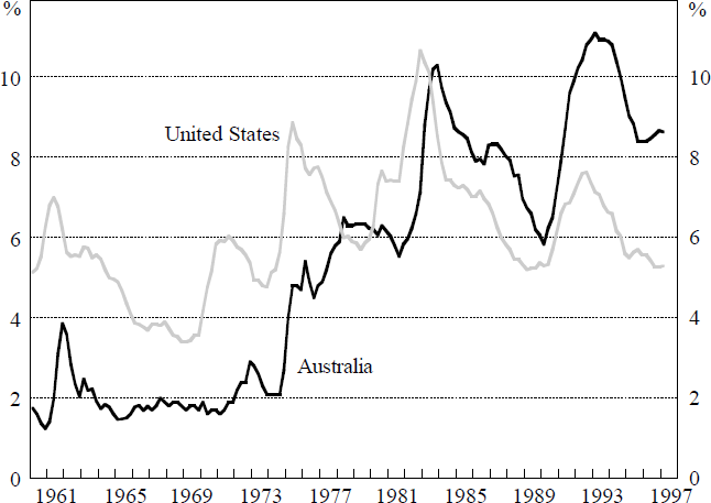
However, all of the models discussed in this section adopt two important assumptions in their estimation which we relax in this paper. Firstly, they assume that the natural rate of unemployment is constant over the sample period, or alternatively that it changes only occasionally by discrete amounts. A comparison of the actual rates of unemployment in Australia and the United States (Figure 1) suggests that the assumption of a constant NAIRU over the sample period may be appropriate in the United States, but it is clearly heroic in Australia. In this paper, we allow the natural rate to vary through time, that is, u^* in Equation (1) is allowed to be time-varying.^[4]

Secondly, the models assume that the Phillips curve specification is linear. Next, we present a specification of a Phillips curve that allows for the possibility that the unemployment gap affects the inflation rate in a non-linear manner.

2.2 Non-linear Model

The non-linear specification that we assume for the Phillips curve is of the following simple form,

A similar specification is included in the TRYM model. In the TRYM model, the NAIRU is determined directly by labour-market factors such as the degree of search effectiveness and institutional features of the wage-determination process. We adopt an alternative approach in our estimation by allowing the information implicit in movements in the inflation rate to help identify shifts in the NAIRU.

The convexity implies that the rise in (unexpected) inflation associated with a positive output gap is greater than the fall in inflation associated with an equally sized negative output gap. Thus, the non-linear specification of Equation (3) captures the implications of a traditional upward-sloping aggregate supply curve. Bottlenecks develop in the economy as the unemployment rate falls below the NAIRU. These bottlenecks result in further increases in aggregate demand (decreases in unemployment) causing ever-increasing rises in inflation. In the limit, as unemployment approaches zero, inflation increases without limit. Note that we have adopted the conservative assumption that this asymptote is reached at zero, when it is likely in reality to be some small positive number. There will be greater convexity in the curve if we use a positive asymptote.

Clark and Laxton (1997) provide a theoretical foundation for a non-linear model of the Phillips curve, using a model of wage and price determination based on that in Layard, Nickell and Jackman (1991).^[5] Roberts (1997) derives similar conclusions from a model of less-than-perfectly rational expectations.

An important implication of a non-linear specification is that there is a distinction between the natural rate of unemployment and the non-accelerating inflation rate of unemployment (NAIRU). This is most easily demonstrated if we assume a slightly different functional form for the non-linear Phillips curve:

where the error term ε_t is distributed normally with mean zero.

As before, the NAIRU is given by u^*. That is, inflation is equal to inflation expectations when the rate of unemployment is equal to u*. However, taking expectations in Equation (4) shows that the average rate of unemployment is given by u^* + var (u_t)/2. We define the natural rate of unemployment to be this stochastic steady state average, which accords with the definition of the natural rate of unemployment given by Milton Friedman in his 1967 American Economic Association Presidential address:

‘The ‘natural rate of unemployment’ … is the level that would be ground out by the Walrasian system of general equilibrium equations, provided there is imbedded in them the actual structural characteristics of the labor and commodity markets, including market imperfections, stochastic variability in demands and supplies, the cost of gathering information about job vacancies and labor availabilities, the costs of mobility, and so on.’ Friedman (1968, p. 8).

Both the NAIRU and the natural rate of unemployment are functions of the institutional structure of the economy. However, the natural rate of unemployment is also dependent on the shocks which affect the variability of unemployment, some of which may be policy-induced.

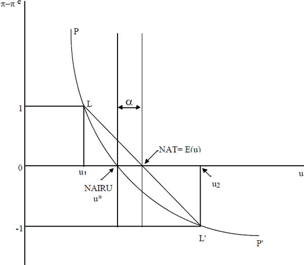
Figure 2 illustrates the general implications of convexity. PP′ is the short-run Phillips curve and u^* is the NAIRU. Comparing the points L and L′ shows that a one percentage point increase in inflation is associated with a smaller gap between unemployment and the NAIRU (u₁ − u^*), than the unemployment gap u₂ − u^* needed to reduce inflation by one percentage point. In this simple world, where the only shocks are +1 percentage point shocks to inflation, the Friedman natural rate of unemployment is the point where LL′ crosses the x-axis. Larger shocks to inflation will shift the line LL′ out, thus increasing α, the difference between the NAIRU and the natural rate.

In the linear framework, the NAIRU and the natural rate are one and the same. Taking expectations in Equation (1), it is clear that the stochastic steady state value of unemployment is the same as u^*, the rate of unemployment where inflation is equal to inflation expectations and is constant. However, in a convex world, the natural rate of unemployment will always exceed the NAIRU. The extent to which it is greater will depend on the variability in the actual rate of unemployment. We discuss the implications of this non-linearity for monetary policy-making in Section 5 below.

Footnotes

Providing another example of Goodhart's Law, Kirby (1981) using data up to 1978 provides evidence of a stable Phillips curve including an estimate of the NAIRU of 2.2 per cent. [3]

Gordon (1997) estimates a version of his traditional linear model with a time-varying NAIRU, using a similar technique to that here. [4]

Dupasquier and Ricketts (1997) also discuss some theoretical foundations for non-linearity. [5]