RDP 1999-01: The Phillips Curve in Australia Appendix D: Technical Issues Involved in Estimating the Kalman Filter

In this appendix we discuss some of the technical issues involved in estimating the NAIRU as a time-varying parameter using the Kalman filter.

Recall that we are treating the NAIRU as a unit root process of the form:

where v_t is assumed to be , and we begin with a price Phillips curve equation which corresponds to Debelle and Vickery's (1997) preferred functional form:

where ε_t is assumed to be N(0,r).

Expanding Equation (D2) gives the following estimating equation:

which can be written more generally as:

where and .

When α is known to be constant we can define a state variable and then Equations (D1) and (D2) constitute a state space form (SSF):

where and var(ε_t) = r.

Because of the ability to represent the equations as a SSF, most researchers using this approach to account for a time-varying NAIRU have estimated the state z_t, conditional upon the past history of y_t (and contemporaneous x_t), with the prediction segment of the Kalman filter. This produces E_t−1(z_t). To do that it is necessary to initiate the recursion with an initial value for the state z_1|0 and its variance z_1|0. In most instances z_1|0 is treated as a parameter and z_1|0 is set to zero (Pagan 1980). Subsequently, conditional upon the values of r, σ_ν and z_1|0 one can derive the innovations η_t = y_t − E_t−1(y_t) and their conditional variances h_t, whereupon the log likelihood will be:

Maximising Equation (D7) then provides a way of estimating any unknown parameters.^[30]

One of the most important parameters to be estimated is q. Apart from fixing it, as Debelle and Vickery do, there have been other suggestions in the literature. Laxton et al (1998, p. 29) report setting q = r when using annual data, because the resulting estimates of the NAIRU were not excessively volatile. This suggests that one needs to study the impact of varying q more carefully in order to understand exactly how the estimates of the NAIRU are made. To do so, it is best to concentrate α and z_1|0 out of the likelihood, leaving only r and q as parameters. The key to doing this is to examine the Kalman prediction equations. One can show that the prediction of the state using past information is:

where K_t = P_t|t−1H_t(H_tP_t|t−1H_t + r)⁻¹ is the gain of the Kalman filter, P_t|t−1 is the variance of z_t conditional on past information (a quantity that is computed by the Kalman filter algorithm and depends only on r and q) and b_t = 1 − H_tK_t. Recursively solving Equation (D8) gives:

where

are also generated recursively for j = 1…n using initial conditions ϕ₁ = 1, s_y1 = 0 and s_x1 = 0.

With this information, the innovations η_t = y_t − E_t−1(y_t) can be written as:

Since the maximum likelihood estimates of α and z_1|0 maximise Equation (D7) it is clear that, for a given r and q, they can be estimated by performing a weighted least squares regression of y_t − H_ts_yt against x_t − H_ts_xt and H_tϕ_t, where the weights are the inverse of the standard deviation of the innovations (their estimated variance h_t depends only on r and q). Thus we can easily concentrate α and z_1|0 out of the log likelihood, leaving only r and q.

The result just described is useful for producing graphical representations of the sensitivity of the log likelihood to variations in q as well as helping us to understand how the NAIRU is estimated. Equation (D8) shows that the estimate of the state z_t is a weighted average of all past values of with weights that decline like b_t but which also vary with K_t. If a linear version of the Phillips curve had been used, H_t would not vary with time, and one could have used the asymptotic version of the Kalman filter; this results in a constant gain K and, hence, constant weights b. In that case one would simply be doing a geometrically weighted average of the residuals when forming the estimated z_t. To derive an estimate of the NAIRU from z_t one also needs to divide by the estimate of γ. This analysis points to the fact that estimates of the NAIRU made using this methodology will depend upon the ability of x_t to predict the change in inflation y_t, and not just on r and q. Moreover, the NAIRU is very sensitive to the estimate made of γ. In this respect, the problems of getting a precise estimate of the time-varying NAIRU are the same as with the constant-NAIRU version in an equation such as Equation (9), where the intercept in the regression is divided by γ. All that happens now is that the numerator is replaced by a weighted average of some residuals rather than an estimated intercept. The explicit formula in Equation (D8) could be useful for those papers looking at monetary policy in the face of a changing NAIRU, for example, Wieland (1998), where the authorities need to solve a signal extraction problem when devising an optimal policy.

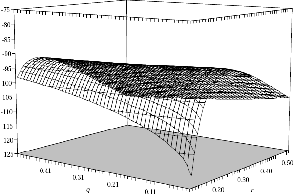
An important message from this analysis is that close attention needs to be paid to devising a suitable specification for the equation linking y_t and x_t. For this reason Equation (9), from Section 2, seems a suitable source of extra regressors in x_t over and above those used by Debelle and Vickery (1997). Such an extension produces the specification for the price Phillips Curve Equation (13), which we estimate in Section 3. Parameter estimates (and the associated t-ratios) for that equation are presented in the text. Here we examine the sensitivity of the log likelihood to variations in r and q using the technique just described. Figure D1 shows a three dimensional plot of the concentrated log-likelihood function against values of r and q. This figure shows that we could accept a wide range of hypotheses about values of q, which means that, for given r, our model is unable to provide a precise estimate of the variation in the NAIRU.

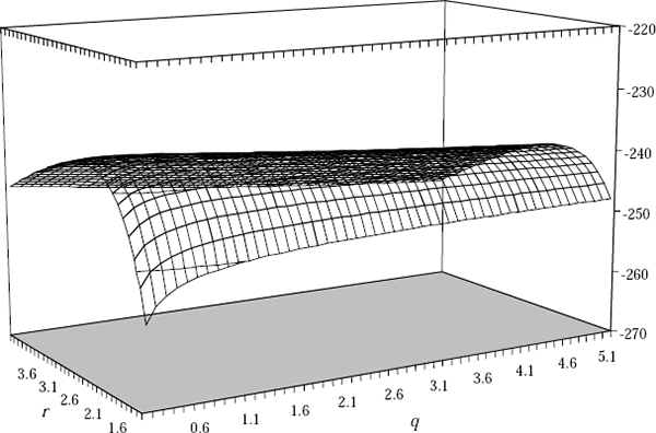
Similarly, for our preferred unit labour cost Phillips curve Equation (14), Figure D2 shows the concentrated log-likelihood function. Here again we see that we could accept a wide range of hypotheses about values of q.

Footnote

Debelle and Vickery (1997) do not proceed in this way. Instead, they set r = 1, pre-specify z_1|0 and P_1|0, and then seem to determine q by how well the resulting estimated path of the NAIRU accords with their priors. Thus, the role of data in determining their NAIRU estimates is more limited than it need be. [30]