RDP 1999-01: The Phillips Curve in Australia 3. Recent Work on the Phillips Curve
January 1999
- Download the Paper 492KB
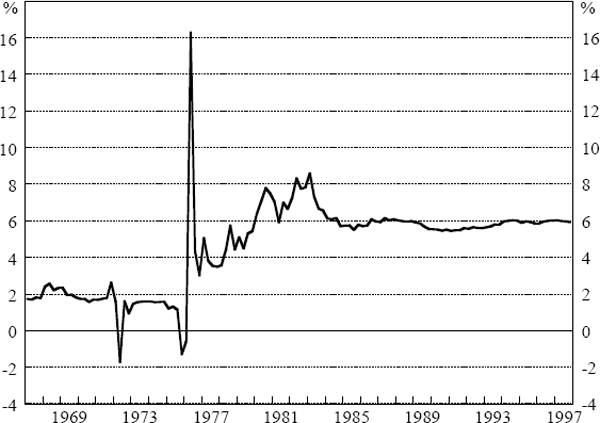
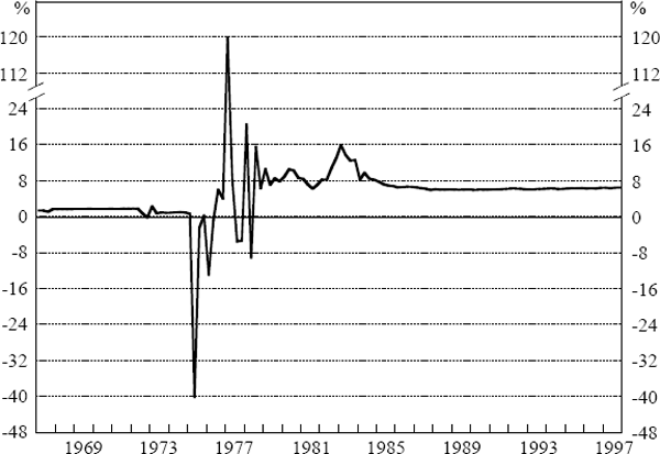
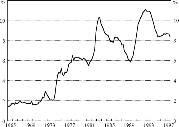
Figures 5 and 6 show recursive estimates of the NAIRU from Equations (9) and (10). Contrasting the beginning and end points reveals quite clearly the shift in the NAIRU, although it appears to have been fairly stable since the early 1980s. These outcomes are consistent with estimates of the NAIRU made in previous research in Australia which had the NAIRU creeping up as data from the early 1970s was included (Borland and Kennedy 1998). Moreover, as seen in Figure 7, the unemployment rate rose sharply in the mid 1970s and has not returned to its pre-1973 level. Consequently, the idea that the NAIRU can be treated as a constant is not very attractive.
If one is to allow the NAIRU to shift over time, then the task becomes one of finding the best way to do that. In Phillips curve specifications such as those estimated earlier, the NAIRU is absorbed into the intercept, presenting the possibility of using statistical procedures to determine the number and location of breaks in that coefficient. Once located, shifts in the NAIRU could be captured by a series of dummy variables. Early work on Treasury's NIF-10 model of the Australian economy did something like this, albeit in an informal way, and the current Treasury macroeconomic model (TRYM) allows for a single shift in the level of the NAIRU in 1974.[14]
The logic of imposing breaks in the NAIRU based on an inspection of the history of the unemployment rate follows from the observation that, within a few years of a shock to the NAIRU, the unemployment rate adjusts back to this new equilibrium level in most macroeconomic models in use in Australia. In the TRYM model, for example, this adjustment takes about three years (Downes and Stacey 1996) and the outcome is similar in the class of models associated with Chris Murphy (Powell and Murphy 1997). Following a shock, the lengthy period of time during which the two series have not converged, however, suggests that it may well be difficult to derive reliable information about the (time-varying) level of the NAIRU simply from the behaviour of the unemployment rate.
There is now an emerging literature (for example, Debelle and Laxton (1997) and the references in Laxton et al (1998)) which involves treating the NAIRU as a unit-root process of the form:

where vt is assumed to be  . The argument for a
unit-root in the NAIRU is apparent from applying ‘unit-root accounting’ to both
sides of Equation (6). The dependent variable in that equation has little persistence; defining
it as yt, an augmented Dickey-Fuller-style regression of
yt against yt−1
and Δyt−j, j = 1…4, gives a
coefficient on yt−1 of 0.53. Since most of the other
variables are in differenced form and Ut behaves like a unit-root process
(Appendix C), this suggests that
. The argument for a
unit-root in the NAIRU is apparent from applying ‘unit-root accounting’ to both
sides of Equation (6). The dependent variable in that equation has little persistence; defining
it as yt, an augmented Dickey-Fuller-style regression of
yt against yt−1
and Δyt−j, j = 1…4, gives a
coefficient on yt−1 of 0.53. Since most of the other
variables are in differenced form and Ut behaves like a unit-root process
(Appendix C), this suggests that  and
Ut must cointegrate. Of course, the variable
and
Ut must cointegrate. Of course, the variable  ln
Pt−1 is quite persistent (0.93 being the first-order term in
the augmented Dickey-Fuller-style regression) and so we expect that this would also be true of
the difference
ln
Pt−1 is quite persistent (0.93 being the first-order term in
the augmented Dickey-Fuller-style regression) and so we expect that this would also be true of
the difference  .
.
For Australia, Debelle and Vickery (1997) use a Phillips curve framework to estimate the NAIRU as a time-varying coefficient using the Kalman filter.[15] Equation (12), which is a modified version of Equation (6), is Debelle and Vickery's preferred functional form for the price Phillips curve (to which we have added an error term εt that is assumed to be N(0, r)).

This equation is a non-linear Phillips curve. Apart from appearing in both of Phillips' original papers (Phillips 1958, 1959) many other estimated Australian Phillips curves have used this non-linear specification, e.g. all those associated with Murphy's models and TRYM. Debelle and Vickery (1997) review the arguments for and against the non-linear Phillips curve specification.
As we have previously discussed, one might expect both import price and speed-limit terms to appear in a price Phillips-curve relationship like Equation (12). This suggests a richer specification, based on Equation (9) from the previous section:
We therefore estimate Equation (13) by maximum likelihood, assuming that the NAIRU evolves as a random walk, as in Equation (11).[16] The coefficient estimates, and associated t-ratios (for the sample period 1966:Q1–1997:Q4) are:

These estimates imply that import prices make a very significant contribution to the acceleration in inflation. Speed-limit effects, while less significant, also seem to contribute.[17] One notable feature of the results is that the magnitude of γ is much smaller than that found with Debelle and Vickery's specification (γ = −1.25), i.e. the influence of deviations of the unemployment rate from the NAIRU upon the acceleration in inflation is much smaller. No doubt part of this is due to the inclusion of the speed-limit term, but it is also due to the fact that other regressors explain variations in inflation movements that were attributed to the NAIRU gap in Debelle and Vickery's specification.
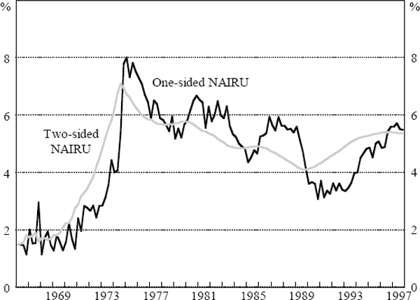
Figure 8 shows both one and two-sided estimates of the NAIRU from Equation (13). For each period, the one-sided estimate is derived using data up to and including the previous period, while the two-sided estimate is based on data from the whole sample. As we would expect, both estimates of the NAIRU rise sharply in the early 1970s. From the mid 1970s until the late 1980s, the estimated NAIRU declines gradually, which may be explained, at least after 1983, as a consequence of the Accord. By the early 1990s, however, the one-sided estimate of the NAIRU has fallen to an implausibly low level, although this problem is less serious when the estimate is based on the whole sample. By the end of the sample, the estimate of the NAIRU is around 5½ per cent, although this estimate is imprecise.[18]
Note that, at a steady rate of both import-price and consumer-price inflation, Equation (13)
implies that a steady unemployment rate will be equal to the NAIRU only when inflation
expectations,  are equal to actual inflation, Δ4ln
Pt−1. Furthermore, while ever inflation expectations exceed
actual inflation, a steady unemployment rate must be above the NAIRU for actual inflation to
remain steady. These are general properties of all the Phillips curves we estimate in this
paper, and also of the Debelle-Vickery Phillips curve. This point is of empirical relevance
because our measure of inflation expectations exceeds actual inflation for extended periods,
with the gap averaging 2.1 per cent per annum over the period 1980–1997 (although it has
disappeared by the end of the sample).
are equal to actual inflation, Δ4ln
Pt−1. Furthermore, while ever inflation expectations exceed
actual inflation, a steady unemployment rate must be above the NAIRU for actual inflation to
remain steady. These are general properties of all the Phillips curves we estimate in this
paper, and also of the Debelle-Vickery Phillips curve. This point is of empirical relevance
because our measure of inflation expectations exceeds actual inflation for extended periods,
with the gap averaging 2.1 per cent per annum over the period 1980–1997 (although it has
disappeared by the end of the sample).
A similar analysis can be carried out by estimating a non-linear version of our unit labour cost Phillips curve, Equation (10), augmented to allow for a time-varying NAIRU:
producing (for the sample period 1966:Q1–1997:Q4):

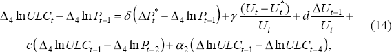
These estimates imply some role for speed-limit effects in the determination of unit labour costs, as they did for the acceleration in price inflation. Figure 9 shows both one and two-sided estimates of the NAIRU from this equation. The unit-labour-cost Phillips curve appears to give a somewhat more plausible picture of movements in the NAIRU than does the price Phillips curve, with much less movement in the estimates of the NAIRU since the mid 1970s. The dip in the unit-labour-cost NAIRU in the mid 1980s also appears more consistent with the timing of the Accord. While there has been considerable debate over whether the Accord reduced the NAIRU, our evidence seems to suggest that it did – at least for some time. At the end of the sample, the NAIRU is estimated to be around 7 per cent, although this number is again estimated imprecisely.
Figure 10 presents a comparison of two-sided (that is, whole-sample) estimates of the NAIRU from our two preferred Phillips curves Equations (13) and (14) and from Debelle and Vickery's price Phillips curve Equation (12). The time-profiles of these three estimated NAIRUs are fairly similar, suggesting that the added complexity of our Phillips curve equations appears to add little to our understanding of the evolution of the NAIRU.
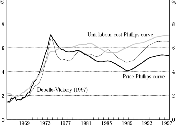
Notes: This figure shows estimates of the NAIRU based in each case on the whole sample of data (two-sided estimates). The Debelle and Vickery (1997) results use their price Phillips curve specification and their methodology estimated over our sample period (1966:Q1–1997:Q4).
There is, however, an advantage to our approach. Debelle and Vickery generate a relatively
smooth time-profile for the NAIRU by imposing the assumption that shocks to the NAIRU
have a small variance (their key assumption is that the parameter q takes the value
0.4, where  and
and  is the variance of
shocks to the NAIRU). However, when the parameters in the Debelle-Vickery system are freely
estimated by maximum likelihood, q takes the value 7.1.[19] Not surprisingly, the
imposed value q = 0.4 is clearly rejected by a likelihood ratio test.
is the variance of
shocks to the NAIRU). However, when the parameters in the Debelle-Vickery system are freely
estimated by maximum likelihood, q takes the value 7.1.[19] Not surprisingly, the
imposed value q = 0.4 is clearly rejected by a likelihood ratio test.
The results generated by maximum-likelihood estimation of the Debelle-Vickery system are, however, unsatisfactory because they imply an unrealistically volatile profile for the NAIRU, with values ranging from less than zero to more than 20 per cent over the sample (results not shown). By contrast, the extra terms in our more complex specifications explain much of the variation in inflation that must instead be attributed to the unemployment gap in the Debelle-Vickery specification. As a consequence, we generate smooth (maximum-likelihood) estimates of the time-profile of the NAIRU without the need to impose restrictions on the parameters which are rejected by the data.
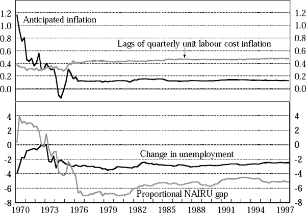
We now examine the stability of our time-varying models of the NAIRU, focusing on our preferred
unit labour cost Phillips curve model Equation (14). The results of recursively estimating the
parameters in that model are shown in Figure 11, where the coefficients on the following
variables are plotted:  (anticipated inflation),
  (proportional NAIRU
gap), ΔUt−1/Ut (change in
unemployment) and Δln ULCt−1 − Δln ULCt−4
(lags of quarterly unit labour cost inflation). The coefficient on the lagged dependent variable
is extremely stable, and so is omitted from the figure. The difficulties that any wage or price
equation faces with data from the early 1970s are very clear, but the equation seems reasonably
stable apart from that.[20]
(proportional NAIRU
gap), ΔUt−1/Ut (change in
unemployment) and Δln ULCt−1 − Δln ULCt−4
(lags of quarterly unit labour cost inflation). The coefficient on the lagged dependent variable
is extremely stable, and so is omitted from the figure. The difficulties that any wage or price
equation faces with data from the early 1970s are very clear, but the equation seems reasonably
stable apart from that.[20]
While treating the NAIRU as a stochastically time-varying coefficient is a useful approach,
there are other ways to deal with the fact that the NAIRU is unobservable. For example, it is
often of considerable interest to know whether unemployment is above or below the NAIRU, without
being so concerned about its distance from the NAIRU. One way to determine this is to treat  in
Equation (6) as a latent variable ξt, and to estimate an equation of the
form:
in
Equation (6) as a latent variable ξt, and to estimate an equation of the
form:

The question then becomes one of how to model the latent variable ξt. One
strategy is to treat it in the same way as Hamilton (1989) and assume that it involves two
states, with the draws in each state coming from different normal densities
N(μ1,σ1) and
N(μ2,σ2).[21]
Transition probabilities then govern the movement from one state to another. Applying this
methodology to the price Phillips curve Equation (13), and replacing  with a two-state latent variable, the resulting parameter estimates, for the sample period
1966:Q1–1997:Q4, are:
with a two-state latent variable, the resulting parameter estimates, for the sample period
1966:Q1–1997:Q4, are:

The signs of the estimated values of μ1 and μ2 are
different, with μ1 being positive. Since γ is expected to
be negative, this sign suggests that the first state occurs when unemployment is below the
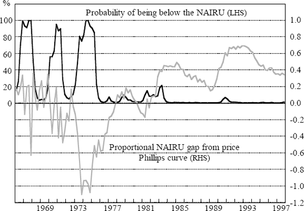
NAIRU. Figure 12 shows the estimated probability of being in this state (below the NAIRU). In
the same figure we also show the proportional NAIRU gap estimated
from the price Phillips curve Equation (13). Figure 12 confirms what has long been believed,
that the late 1960s and early 1970s were periods when the economy was below the NAIRU, but,
apart from a period at the beginning of the 1980s, the Australian economy has since been above
the NAIRU.
Making the NAIRU a strictly exogenous variable as in Equation (11) means that OLS can be applied under the same conditions as when the NAIRU is assumed fixed.[22] However, as there has been a great deal of debate over determinants of the NAIRU, it seems worthwhile to experiment with some modifications to Equation (11). Specifically, we estimate models of the form:

where the factors f1t and f2t are taken to be I(1) and are therefore entered in differenced form. Two I(1) variables which are thought to influence the NAIRU are the replacement ratio and the long-term unemployment rate (Figure 13). The latter is taken to represent ‘hysteresis’ effects. After jointly estimating Equation (14) with the augmented specification for the NAIRU in Equation (16), the coefficients a1 and a2 are found to be neither statistically nor economically significant. Other experiments in which the factors were taken to be the lagged values of the unemployment rate itself produced the same conclusion.
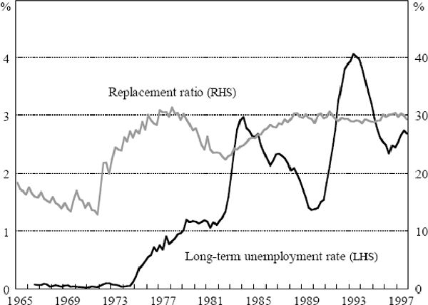
Our inability to explain changes in the NAIRU using either the replacement ratio or the long-term unemployment rate, while disappointing, accords with international studies which have also found it difficult to explain differences in unemployment rates between countries and across time on the basis of a small number of measurable, causal factors (Jackman 1998).
Footnotes
We formally tested for breaks in our Phillips curve relations, Equations (9) and (10), by applying the battery of tests in Bai and Perron (1998). Generally, these tests suggest one or two breaks in each relation. For the price equation, the breaks are in 1972:Q4 and 1974:Q4. However, given how close these are to one another, it seems best to regard them as a single break around 1973. For the wage equation, the most significant break identified was in 1977:Q2 with a less significant break in 1973:Q4. Thus, the time pattern of the NAIRU evident in the recursive estimates shown in Figures 5 and 6, seems to hold up to more formal testing. [14]
Given the fact that the Kalman filter does make some normality assumptions, and the change in inflation is clearly non-normal (Figure 2), one might wish to be cautious when interpreting the results from this estimation. [15]
Appendix D provides a discussion of some of the technical
issues involved in this estimation. Two changes were made to the specification in
Equation (9). One was to make the speed limit term – the lagged change in
unemployment – a ratio of the unemployment rate, in line with the non-linear
structure of the Phillips curve. The second was to use the unemployment rate rather than
a moving average of it when defining the excess demand variable. As was mentioned
earlier, from the point of view of fit, it matters little whether one uses
MA4(Ut) or Ut as the measure of
unemployment, and the former was preferred earlier because it improves the shape of the
implied lag distributions to a temporary shock. However, it would be difficult to work
with  in the context of the Kalman filter. We also estimated
models in which the Phillips curve was linear in the unemployment rate but, based on the
values of the maximised log likelihoods, such models were always rejected in favour of
the non-linear versions.
[16]
in the context of the Kalman filter. We also estimated
models in which the Phillips curve was linear in the unemployment rate but, based on the
values of the maximised log likelihoods, such models were always rejected in favour of
the non-linear versions.
[16]
Debelle and Vickery (1997) also tested for speed-limit effects, but generally found them to be of the wrong sign (and insignificant). This result is presumably a consequence of the omission of other relevant inflation explanators from their equation. [17]
The final estimate of the NAIRU is sensitive to the parameters γ and σν. Since both are estimated imprecisely, with t-ratios less than 2, the NAIRU is also estimated imprecisely. [18]
Other parameters also take different values, but the value of q is the key difference. [19]
An alternative approach for testing the structural stability of the equation is to apply the tests described in Bai and Perron (1998). These tests suggest that there may be a structural break, although their sequential test suggests no break. [20]
Another would be to allow the gap between the unemployment rate and the NAIRU to evolve as an autoregressive process. [21]
A stochastically varying NAIRU also makes it computationally difficult to treat the unemployment rate as an endogenous variable in a (possibly) non-recursive system. Thus the type of analysis conducted by King and Watson (1994) is difficult to perform unless one conditions upon estimates of the NAIRU, but doing so fixes one of the equations of the system. [22]