RDP 1999-01: The Phillips Curve in Australia 2. Early Studies of the Australian Phillips Curve
January 1999
- Download the Paper 492KB
Phillips curve research within Australia can be usefully encapsulated within the context of the following three equations:
In Equation (1), Pt is the consumer price level excluding interest rates and
other volatile items, and its rate of change is the underlying inflation rate, until recently
the series targeted by the Reserve Bank of Australia.[1] ULCt is
unit labour costs and PMt is tariff-adjusted import prices. The presence of
import prices reflects the fact that a significant proportion of goods consumed within Australia
are imported and that the cost structure of Australian industry is affected by imported goods as
well.[2] The second
of the equations describes the evolution of unit labour costs. In most studies of the Phillips
curve that have concentrated on labour compensation, ULCt is decomposed into
its components of wages and productivity growth. Wage movements, or more broadly unit labour
costs, are driven by expectations of the price level  , by ‘demand
factors’ zt, and ‘other’ factors
x2t. Finally, expectations are modelled by combining a
backward-looking component and some other (possibly forward-looking) measure,
x3t. The unit of observation is usually a quarter (since both price
and wage data are available with that frequency) and the choice of k
in Δk determines the period over which wage and price movements are
measured. Setting k = 4 produces annual wage and price movements.
Phillips' (1959) Australian version of his classic paper estimated a wage version of Equation (2) with quarterly data and k = 4.[3] However, compared with his British work there were some significant changes, mostly in response to the institutions governing the way in which Australian wages were set. Until the 1990s, wage setting in Australia was quite centralised and distinctive. A legal system set award and minimum wages for most industries and ‘collective bargaining’ amounted to unions and employers arguing cases before an Arbitration Court, which made decisions regarding award wage changes. Thus, the equations Phillips presented were based on wage inflation that was closer to ‘award wages’ than actual ‘earnings’; the difference, frequently referred to as ‘earnings drift’, arose from strong unions' capacity to negotiate above-award wages outside the Arbitration Court system. His equations also featured unemployment as well as import and export price inflation. The influence of the institutional features upon his thinking was particularly evident in the comments he made about the effects of the latter upon wages:
It seems that the decisions of the Arbitration Court were strongly affected by the rapidly rising export prices… (Phillips 1959, p. 3)
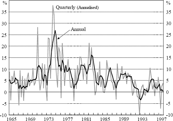
The importance of the courts in determining wage inflation in Australia was manifested in many ways. As well as cases relating to specific industries, one had ‘National Wage Cases’ in which the whole structure of awards was generally adjusted upwards. The table in Appendix A details the outcomes of each of these National Wage cases between 1968 and 1981 (the end of wage indexation in Australia) and also gives the change in average earnings in the year after each decision came into effect. The exact timing and magnitude of these decisions rendered quarterly movements in wages very erratic, which even conversion to annual changes could not entirely smooth out (Figure 1). Such a series, particularly the quarterly one, may be hard to model.

Two responses could be made to the erratic movements evident in Figure 1. First, one might treat the Phillips curve as determining prices rather than wages. Pitchford (1968) seems to have been the first to do this in Australia, although it had been popular in the US for some time. A useful benchmark Phillips curve involving price inflation, that we will frequently refer back to later, is constructed from the following two equations:
where  is a
measure of expected inflation and zt measures ‘excess demand’.
Almost all of the early work on the Phillips curve in Australia (including Phillips (1959))
accepted that there was a trade-off between inflation and unemployment, even in the ‘long-run’.
In the early 1970s, however, this proposition was increasingly questioned and a lot of time was
spent testing whether a long-run trade-off actually existed, i.e. whether ϕ = 1.
As we discuss later, Michael Parkin was an influential figure in that debate and Chart 1 in
Parkin (1973, p. 135) suggests that the estimates made of ϕ had been slowly
converging on unity.[4]
Henceforth, we assume that ϕ = 1. Doing so, and replacing zt
with the difference between the unemployment rate Ut and the NAIRU
  , enables us
to reparameterize Equations (4) and (5) as:
Furthermore, if the NAIRU is constant, Equation (6) may be re-written as:
where α = −γU*.
Equation (6) is a useful specification which we will retain in later work. By making the acceleration in inflation the dependent variable, the equation becomes one that involves an ‘accelerationist’ form of the Phillips curve. If the NAIRU is constant, U* can be treated as a parameter and then Equation (6) can be estimated as a non-linear regression (alternatively, Equation (7) could be estimated as an OLS regression and U* recovered from the estimated parameters a and γ).
To estimate Equation (6), we first replace Ut with MA4(Ut),
where MA4 is a fourth-order moving-average operator.[5] Second, we use
inflation expectations computed by Debelle and Vickery (1997) from bond yield data to represent
 .[6] In this, and all
subsequent estimations, log levels and their differences are multiplied by 100. Estimating
Equation (6) as a non-linear regression over the period 1965:Q2–1997:Q4 gives (with
absolute values of t-ratios in brackets):
While the signs are as expected, the fit is very bad, with R2 = 0.09 and DW = 0.91. Moreover, fitting the relation over the sub-period 1965:Q2–1976:Q1 generates an estimate of U* = 2.2%, indicating that the relation has not been particularly stable.
Table 1 summarises early research on wage and price Phillips curves in Australia. When it came to modelling wage inflation, rather than price inflation, researchers in policy institutions mostly examined movements in labour costs conditional upon the decisions taken by the Arbitration Court. Technically, x2t in Equation (2) was set to changes in award wages and what was modelled was essentially ‘earnings drift’, that is, the gap between award wages and those actually paid; something likely to be affected by the state of the labour market. Some of these studies are also summarised in Table 1. Of course, such a ‘solution’ was less helpful in a forecasting environment as some prediction needed to be made about future Arbitration Court decisions, i.e., an equation for x2t was necessary. There were a number of attempts to do this and Higgins (1973) and Jonson, Mahar and Thompson (1973) were among the earliest of these studies. Generally, modelling of earnings given award wages was quite successful. In contrast, it was difficult to model either earnings without conditioning upon award wages or award wages themselves. Given the frequency of Arbitration Court decisions, it was probably inevitable that annual wage movements (k = 4) became the preferred series to model.
| Author(s) | Dependent variable | Excess labour demand variable(s) | Other variable(s) |
|---|---|---|---|
| Phillips (1959) | Annual % change in wages | 1/U2 |
|
| Hancock (1966) | Annual % change in wages | lnU, ΔlnU |
|
| Schott (1969)(a) | Level of wages | Level U, V |
|
| Jonson (1972)(a) | Annual % change in wages | 1/U |
|
| Parkin (1973)(a) | Annual % change in wages | 1/U, Δ(1/U), V − U |
|
| Higgins (1973) | Annual % change in wages | V/U, Δ(V/U) |
|
| Jonson, Mahar and Thompson (1974)(a) | Annual % change in wages | V/U, Δ(V/U) |
|
| Carmichael and Broadbent (1980)(a) |
Quarterly % change in wages | V − U |
|
| Kirby (1981) | Quarterly % change in wages | U |
|
| Gregory (1986) | Quarterly % change in wages | U, V, O |
|
| Simes and Richardson (1987) | Quarterly % change in wages | U, O |
|
| Price equations | |||
| Pitchford (1968) | Annual % change in prices | V − U |
|
| Nevile (1977) | Annual % change in prices | U, V − U |
|
Notes: U is the unemployment rate (or level, where
indicated). |
|||
Equation (8) is an equation for unit labour costs that parallels the ‘price equation’ in Equation (6):
Estimates of its parameters over the period 1965:Q2–1997:Q4 are:
with R2 = 0.23 and DW = 0.49.[7] By and large, the effects are better determined than in the price equation. However, the instability in the price equation is also present in the wage equation, with an estimated NAIRU over the earlier sub-sample (1965:Q2–1976:Q1) of 2.5 per cent.[8]
How might one improve upon the specifications of these two Phillips curve equations? As mentioned earlier, it is unlikely that one could capture the impact of import prices upon final goods prices with what is effectively just wage pressures. Moreover, there may be ‘speed-limit’ effects, so that a rapid change in the unemployment rate has an impact on prices, implying that the demand measure might also include changes in the unemployment rate. Finally, there is a decision to be made about whether to model quarterly or annual movements in wages and prices. We choose to model annual movements, which leads us to the following specification for the change in annual price inflation:[9]
Since the dependent variable in this equation is the change in annual inflation, the augmented list of regressors is extended to include ΔlnPt−4. When the four lagged quarterly inflation rates are added to the regressor set we find that ΔlnPt−1 and ΔlnPt−4 had close to equal and opposite signs, accounting for the formulation shown. The import-price inflation term was also entered in the specific way described, as that was an acceptable simplification of more complex dynamics.[10] One advantage of this specification is that it ensures that the estimate of the NAIRU is independent of the steady-state rate of either domestic or imported inflation.
Estimating Equation (9) over the sample period 1965:Q3–1997:Q4 produces the following estimates:
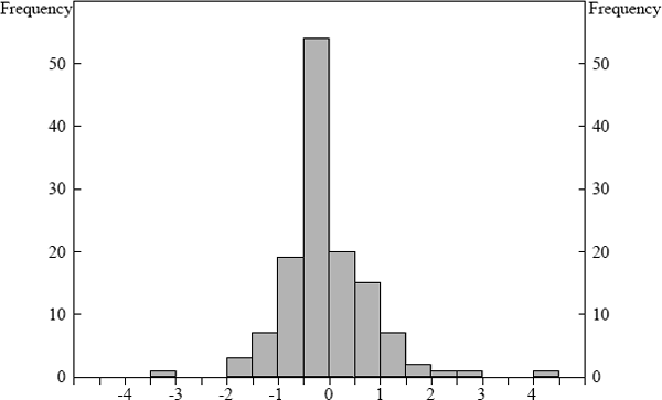
The R2 = 0.67, DW = 2.29 and the χ2(4) statistic for testing that the first four serial correlation coefficients are zero is 10.48 (p-value = 0.03). Normality of the residuals is very strongly rejected, the Jarque-Bera test giving a value of 220. The reason for this becomes clear by plotting the histogram of the dependent variable (Figure 2). Like many financial asset prices there are too many small movements in the acceleration in inflation for this variable to be treated as normally distributed.

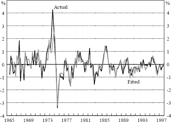
The fit of the equation is quite impressive. Looking at the fitted and actual values in Figure 3, one sees that the very strong movements of inflation in 1974 defeat it, but apart from that, the equation produces quite a good fit. The implied natural rate over the period is 5.95 per cent with a standard error of 1.19 per cent. However, there are some less attractive aspects of the equation. The most important one stems from the low estimated coefficient on the unemployment rate, which implies that the direct effects of deviations from the NAIRU account for a relatively small amount of the movements in annual inflation. Thus, a 3 percentage point departure from the NAIRU would only cause a change in annual inflation of 0.12 per cent in the next quarter. This is a small number when compared with the maximum increases and decreases in the sample, which were 4.26 per cent and −3.37 per cent. The very small estimated coefficient δ implies that inflation expectations are predominantly backward looking, while the non-zero value for d supports the idea that there are speed-limit effects on inflation.

It is interesting to use a similar specification to explain annual real unit labour cost inflation.[11] However, in light of the different dependent variable, the specification is adjusted in two ways: import prices are removed and a lagged dependent variable is added based on its significance in the equation (the corresponding variable did not appear in the price equation because it was insignificant). Specifically, we estimate:
over the sample period 1965:Q3–1997:Q4, producing:
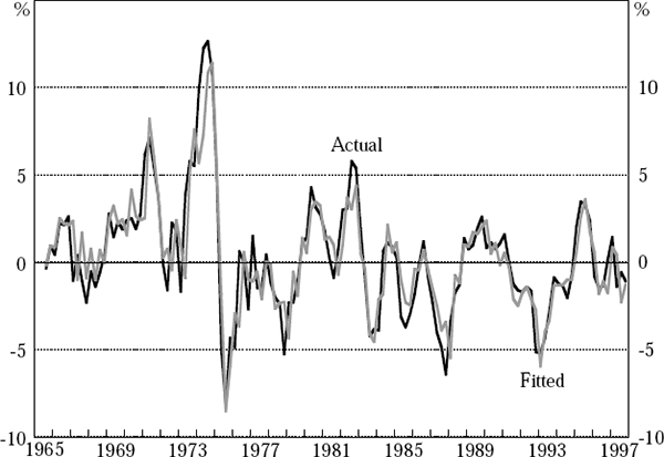
The R2 = 0.80, DW = 2.29 and the χ2(4) test statistic for serial correlation is 9.90 (p-value = 0.04). The Jarque-Bera test for normality of the residuals has a value of 14.85.[12] The estimated NAIRU is 6.58 per cent with a standard error of 0.81 per cent. Figure 4 shows the actual and fitted values of the dependent variable from this equation. Generally, the fit of the equation is quite good and tends to be superior to that of the price equation. Given the history recounted earlier about the difficulty of modelling wages, it is perhaps a little surprising that the equation works so well compared with the price equation. One difference between our work and most of that in the past is that we model unit labour costs rather than wages. Since unit labour costs are relevant to pricing decisions, focusing on them seems a reasonable strategy. Our use of a longer sample period than was available in earlier studies may also be relevant since the wage-setting process has become less regulated over time, especially in the 1990s.[13]

Note: * Unit labour cost inflation deflated by lagged price inflation.
Footnotes
As discussed later, the Reserve Bank has a target for inflation of 2–3 per cent per annum on average over the medium term. This target was expressed in terms of underlying inflation until October 1998. [1]
Gali and Gertler (1998) effectively consider a model in which Pt is a mark-up over ULCt. In our data set ln Pt and lnULCt are I(1) processes and a dynamic equilibrium mark-up model would naturally be formulated in an error correction form. In this case, Equation (1) would include an error correction term which could be interpreted as the labour share of income. de Brouwer and Ericsson (1995, 1998) include such a term in their model of Australian inflation, but over our sample period this term does not appear to be stationary. Moreover, when it is added to the Phillips curve equations which we estimate in Section 3, it is of marginal significance. [2]
Perry (1980) and Pitchford (1998) provide good discussions of this paper. [3]
The proposition that ϕ = 1 could be tested because the relevant studies
modelled wages rather than prices. Given any information set used by agents, one could
replace Δκ ln  with Δκ ln Pt and then
instrument Δκ ln Pt with elements of
that set, provided the instruments were not correlated with the error term of the wage
equation. To ensure this, the minimal information set was assumed to be composed of
award wages, overseas prices and productivity movements (in fact, instrumental variables
estimation was rarely performed directly but rather these three instruments were
substituted for the actual inflation rate and a restriction was imposed upon the three
weights, that they added to unity, thereby reducing the three unknown weights to two).
It was therefore possible to avoid the Lucas/Sargent critique by working with a wage
equation (a strategy that would clearly fail if one had price rather than wage inflation
as the dependent variable). We do not comment further on this debate here.
[4]
If one does not do this then a transitory rise in the unemployment rate will have a peculiar effect upon quarterly inflation rates due to the fact that the annual inflation rate is just the sum of the quarterly inflation rates. Specifically, these would fall in the first quarter then rise in subsequent quarters. In practice, it makes almost no difference to the point estimates whether we use Ut or MA4(Ut) as the Ut series is already very smooth. Many studies have used MA4(Ut), e.g. Jonson, Mahar and Thompson (1973). [5]
Appendix E contains descriptions and the sources for the data which we use in this paper. [6]
Because the Phillips curve is a single equation in a system, our estimates of Equations (6) and (8) are based on some exogeneity assumptions. Appendix B contains a discussion of the exogeneity assumptions relevant to estimating Phillips curves. [7]
One response to this instability by earlier researchers was to experiment with different measures of demand pressure. Stimulated by the emerging literature on the role of ‘insiders’ and ‘outsiders’ in the wage-setting process, a range of these demand pressure variables have been proposed. For example, Gregory (1986) looked at overtime hours worked while Cockerell and Russell (1995) constructed a measure of ‘inside unemployment’. Neither of these alternatives produces much of an improvement in our equations though; with overtime the crucial fit statistics are R2 = 0.19 and DW = 0.53, while using inside unemployment results in R2 = 0.23 and DW = 0.60. [8]
As observed previously, annual movements were favoured in early work on the Phillips curve but, after Kirby (1981), there was a shift towards modelling quarterly wage and price movements. From an economic viewpoint, it is of more interest to explain annual movements in inflation than quarterly movements. This explains our choice of dependent variable in Equation (9). Consider deriving Equation (9) from an equation that has quarterly inflation (Δln Pt) as the dependent variable and three lagged changes in quarterly inflation (Δln Pt−j, j = 1…3) as regressors. These regressors have associated coefficients φj. Since annual inflation is the sum of four consecutive quarterly price changes, changing to annual inflation as the dependent variable simply means that the regressors Δln Pt − j now have coefficients (1 + φj). In an equation with annual inflation as the dependent variable, the coefficients on these regressors can be freely estimated, and any restrictions upon the φj can be tested and imposed. [9]
Since the import price index is constructed from the contemporaneous exchange rate which
we would expect to appear as the last variable in any recursive system, it is natural to
exclude PMt from Equation (9) and only allow lagged values of that
variable to enter the equation.
Research in Australia points to a strong
relationship between the terms of trade and the exchange rate (Gruen and Dwyer 1996).
Moreover, movements in the terms of trade tend to be dominated by variations in
foreign-currency denominated export prices. Thus, by excluding PMt
from the equation, we are implicitly assuming that the impact of export prices upon the
price level within the quarter is quite small, which is consistent with Gruen and Dwyer's
results.
[10]
The variable being explained is not strictly movements in real unit labour costs, since the deflator is the price level in the previous period rather than the current one. [11]
The Jarque-Bera test implies that this equation's residuals are also non-normal. In contrast to the price equation, however, this is caused by the influence of a few quarters of large rises in the dependent variable (which coincide with large wage-case decisions) rather than the presence of many small movements. Excluding these observations, normality of the unit-labour-cost residuals cannot be rejected. [12]
One test of the importance of the longer sample period is to see how well the equation performs over a sample finishing in 1973:Q1. The answer is that, in this regression, all of the variables are insignificant apart from the wage inflation variables. We are, of course, only using 31 observations in this regression and so no precision could be expected. By contrast, however, when the sample is restricted to the last 31 observations, all of the variables are significant, with the exception of the change in unemployment. [13]


