RDP 2008-04: A Small BVAR-DSGE Model for Forecasting the Australian Economy 3. Data and DSGE Priors
September 2008
3.1 DSGE Priors
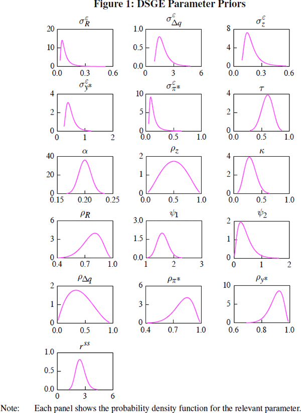
The priors for the DSGE parameters are given in Table 1 and Figure 1. These differ
from those in Lubik and Schorfheide (2007), who apply their model to four
countries, and vary only a small subset of the priors for each country. Our
priors are selected in part by examining the results of recent DSGE modelling
for Australia and by reference to economic theory. Additionally, we draw on
past experience in modelling the Australian economy at the Reserve Bank of
Australia. However, for many parameters, the differences between our priors
and theirs are small. Rather than place a prior on the discount factor, we
place a prior (and estimate) the steady-state (real) interest rate rss. Note that  . The standard deviations
of the five structural shocks are denoted
by
  .
.
| Parameter | Distribution | Mean | Standard deviation |
|---|---|---|---|
| Households and firms | |||
| ρ | Beta | 0.6 | 0.1 |
| α | Beta | 0.2 | 0.011 |
| rss | Gamma | 2.5 | 0.5 |
| Phillips curve | |||
| Κ | Beta | 0.3 | 0.1 |
| Taylor rule | |||
| ρR | Beta | 0.77 | 0.1 |
| Ψ1 | Gamma | 1.6 | 0.2 |
| Ψ2 | Gamma | 0.4 | 0.25 |
| Exogenous persistence | |||
| ρΔq | Beta | 0.4 | 0.2 |
| ρπ* | Beta | 0.8 | 0.1 |
| ρy* | Beta | 0.9 | 0.05 |
| ρz | Beta | 0.5 | 0.2 |
| Exogenous shock standard deviations | |||
 |
Inverse gamma | 0.1 | 0.2 |
 |
Inverse gamma | 1.9 | 0.8 |
 |
Inverse gamma | 0.2 | 0.1 |
 |
Inverse gamma | 0.5 | 0.2 |
 |
Inverse gamma | 0.15 | 0.15 |

The priors we place on the standard deviations of the structural shocks are tighter and have lower mean values than those in Lubik and Schorfheide (2007).[11] This reflects our view that the structural shocks probably were quite moderate for much of the sample period for the Australian economy (1993 onwards; see Section 3.2). For example, we suspect that monetary policy shocks have generally been small in magnitude during the inflation-targeting regime. The mean of our prior on the standard deviation of terms of trade growth shocks is higher than that set for the other shocks, to account for the apparent volatility of this series.
Turning to the structural parameters of the DSGE model, our prior for the import share of consumption (α) has the same mean as used by Lubik and Schorfheide (2007), namely 0.2, but is considerably tighter, reflecting that over the estimation period the import share of GDP was around this value (and that output equals consumption in this model). The mean of the prior for the intertemporal elasticity of substitution (τ) is 0.6, which is larger than the mode used by Nimark (2007) (0.3), but less than the mean value of Justiniano and Preston (forthcoming) (0.8). The parameter κ, together with α and τ, determines the slope of the Phillips curve. We select the mean of the prior for κ so that (given the priors of these other parameters) it implies a similar slope to that estimated by Kuttner and Robinson (forthcoming) using GMM over the inflation-targeting period.
For the parameter ψ1 in the Taylor rule (Equation (6)), which describes the monetary policy reaction to deviations of inflation from its steady state, the probability mass is distributed over values greater than one. This ensures that the real interest rate increases in response to higher inflation (that is, the Taylor principle is satisfied). Further, consistent with previous studies – which tend to find a considerable degree of interest rate smoothing (for example, de Brouwer and Gilbert 2005) – we place a large prior on the parameter ρR.
3.2 Data
There are five observable variables in the model: growth in chain-volume non-farm GDP (Δyobst); the quarterly average cash rate (Robst); trimmed-mean consumer price index (CPI) inflation (πobst); the change in the inverse of the nominal trade-weighted exchange rate (Δobst) (consequently, negative values correspond to an appreciation); and growth in the terms of trade (Δqobst) – that is, the ratio of export to import prices. The data sources are given in Appendix B. We multiply log differences (for example, non-farm output) by 100, so as to approximate percentages.[12] We de-mean all of the data as the DSGE model variables are in terms of log deviations from steady state. The estimation sample is from 1993:Q1, when inflation targeting began in Australia, until 2007:Q4.
3.3 Measurement Equations
The measurement equations, given below, map the observed data (yt, which are also the variables in the VAR and are on the left-hand side below) into the model variables (shown on the right-hand side):
Recall that in the DSGE model, output has been normalised by technology. Consequently, observed output growth is related to both output and technology growth as per Equation (10). The cash rate is expressed on a per annum basis, whereas the model interest rate is the gross one-period return. Also, as we have log-linearised the model (about its steady state), Rt more precisely is the log deviation of the gross rate from its steady state.


