RDP 2008-10: Solving Linear Rational Expectations Models with Predictable Structural Changes 4. Numerical Examples
December 2008
- Download the Paper 311KB
4.1 The Model
We illustrate the solution method outlined above with a series of examples using
a version of the New-Keynesian model presented in Ireland (2007). Unlike Ireland,
we assume, for simplicity, that the gross inflation target is a policy-determined
constant, that the deviation of the technology process from its steady state,
 ,
follows a stationary process, and that there are no habits in consumption.
Under these assumptions it is easy to show that the equilibrium obeys the
following set of log-linear equations
Equations (21), (22), (23) and (24) are the ‘IS-curve’, Phillips curve,
Taylor rule, and definition of the growth rate of output, while (25), (26),
and (27) govern the behaviour of the exogenous shock processes to demand,
 ,
the mark-up,
  , and technology,
  . πt
is the log gross rate of inflation between periods t − 1 and
t; π* stands for the log of the target rate
of inflation;
  is the percentage deviation of output from
its steady-state level, Y;
  is the growth rate
of output; rt = lnRt stands for the
log of the gross nominal interest rate between periods t and t
+ 1; r = π* − ln β is
the steady-state level of rt; β is the household's
discount factor; σ is the inverse of the intertemporal elasticity
of substitution; α ∈ [0,1] governs the degree to which
price-setting is ‘backward-looking’; the parameters ρa,ρe
and ρz all ∈ [0,1); and ψ = (θ
− 1)/φ is defined for convenience, where θ
is the steady-state elasticity of substitution between intermediate goods and
φ controls the magnitude of price adjustment costs. Finally,
εa,t,εe,t,εr,t
and εz,t are all assumed to be
independent and identically distributed (iid) disturbances with mean
zero and standard deviations σa, σe, σr,
and σz respectively.
While some variables are expressed in percentage deviations from their steady-state values, others, like πt and rt, are left expressed in log-levels. The only reason for this is that it aids in the interpretation of the numerical examples that follow – in particular, those that involve changes in the steady-state values of these same variables. For example, a change of the inflation target alters the steady-state values of inflation and the nominal interest rate.
Equations (21) to (27), together with the definitions for the one-period-ahead forecast errors can be easily put in the form Γ0yt = C + Γ1yt−1 + Ψεt + πηt.
We set the model's parameters to obtain a benchmark calibration for the numerical examples that follow. The parametrisation (Table 1) is inspired empirically and in cases borrows values from the literature of similarly estimated models. The parametrisation itself is, for our purposes, unimportant.
| Parameter | Description | Value |
|---|---|---|
| π* | Inflation target | 0.0125 |
| β | Household's discount factor | 0.9925 |
 |
Intertemporal elasticity of substitution | 1.0 |
| α | Backward-looking price-setting | 0.25 |
| ψ | Elasticity of substitution adjusted for price adjustment costs | 0.1 |
| ρr | Persistence of nominal interest rate | 0.65 |
| ρπ | Policy rule inflation coefficient | 0.5 |
| ρy | Policy rule output gap coefficient | 0.1 |
| ρg | Policy rule output growth coefficient | 0.2 |
| ρa | Persistence of demand shocks | 0.9 |
| σa | Standard deviation of demand disturbance | 0.02 |
| ρz | Persistence of technology shocks | 0.9 |
| σz | Standard deviation of technology disturbance | 0.007 |
| ρe | Persistence of mark-up shocks | 0.9 |
| σe | Standard deviation of mark-up disturbance | 0.001 |
| σr | Standard deviation of monetary disturbance | 0.002 |
4.2 An Increase in ρπ
We start by considering the impact of announcing a more aggressive policy towards inflation. The announcement refers to the future value of ρπ. In particular, the two structures differ only with respect to their value of ρπ. Both structures, however, share the same steady state. The initial structure is that of the benchmark parametrisation, which sets ρπ to 0.5. The final structure sets ρπ to 1.
The announcement of a different future value for ρπ has no effect on the evolution of the non-stochastic steady state; the dynamics are uninteresting if the system begins and remains at its steady state. To study the implications of an anticipated structural change we consider a persistent demand shock and assume that the economy is away from its steady state when this information is known.
Figure 1 shows impulse responses of output, inflation, the nominal interest rate, and output growth to a one standard deviation demand shock, εa,t. The green lines show conventional impulse responses given the initial structure: the impulse responses that would have prevailed in the absence of any known future change in policy. Similarly, the orange lines show the conventional impulse responses under the final structure: the responses that would have prevailed had the new rule always been in place. The blue lines show the equilibrium responses of a credible announcement made in period 4 that in period 8 a new policy that sets ρπ equal to 1 would be in place.
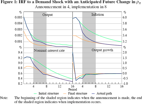
For the first three periods, the economy behaves according to the initial structure. At the time of the announcement, inflation, output and the interest rate jump to their new SSP. Because of forward-looking price-setting behaviour, the credible announcement of a more aggressive policy towards inflation in the future serves to reduce inflation relative to the response in the absence of any announcements. In period 4, annualised inflation would have been around 5.7 per cent, but the announcement has the effect of bringing inflation down to 5.5 per cent. In period 7, prior to the actual implementation of the new policy rule, inflation is already around 5.2 per cent, close to where inflation would have been had the final structure always been in place.
The way the economy evolves between the announcement and the implementation is essentially a function of the length of the intervening period and also of the ‘distance’, so to speak, between the initial and final reduced forms. If, for example, the announcement involves a change which is far into the future, then its contemporaneous impact would be small. In fact, for the first few periods the economy's response would be fairly similar to those of the prevailing structure. This is illustrated in Figure 2 which compares the response of inflation in Figure 1 with the one that would prevail if the new policy is implemented in period 24 (instead of period 8).
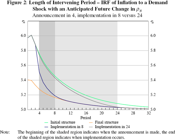
The more the announcement alters the future reduced form of the system, relative to its present one, the more strongly the economy reacts in the intervening period.
4.3 A Change of the Inflation Target
We consider the impact of announcing a lower inflation target. The announcement refers to the future value of π*. As before, we assume that a demand shock hits the economy in period 1 and that at the beginning of period 4 the central bank announces that it will implement a lower inflation target from period 8 onwards. In this case, notice that the two structures differ only with respect to the steady-state value of their nominal quantities. The impulse response functions for output are invariant to the level of the inflation target (Figure 3). However, because of the presence of nominal rigidities, the announcement has real effects.
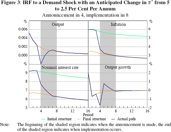
As Figure 3 shows, both inflation and output fall after the announcement is made. The central bank conducts policy as governed by the initial policy, however, which implies a departure of inflation to well below its initial inflation target. Although the central bank cuts the nominal interest rate, the real interest rate increases and output growth consequently falls.
4.4 Announced Shocks
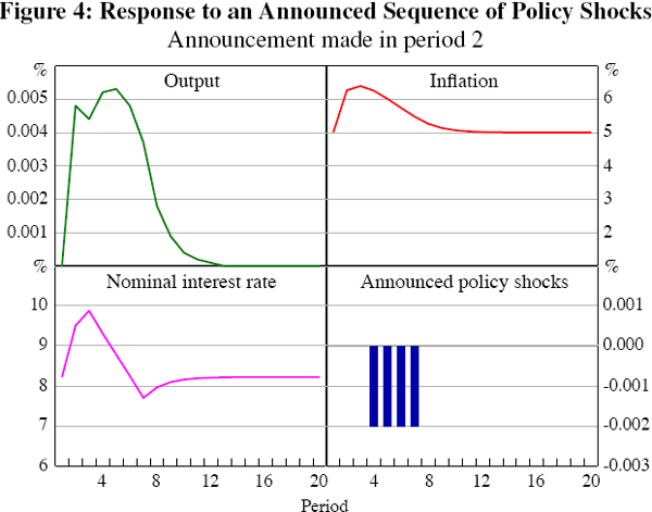
Figure 4 shows the responses of output, inflation and the nominal interest rate to an announced sequence of monetary policy shocks (as shown in the bottom right panel). In period 2, the monetary authority announces that a sequence of deviations from the prevailing rule will occur. In particular, these are expansionary shocks to the policy rule and consequently inflation and output increase in the announcement period. Inflation and the nominal interest rate reach their peaks in period 3 before the announced shocks take place. Unlike the case with unanticipated shocks, as these fully anticipated shocks occur, output, inflation and the nominal interest rate are already gradually returning towards their steady-state values.
4.5 A Stochastic Simulation: Announcing a New Monetary Policy Rule
As we have discussed above, the solution method described in Section 3 can be used recursively
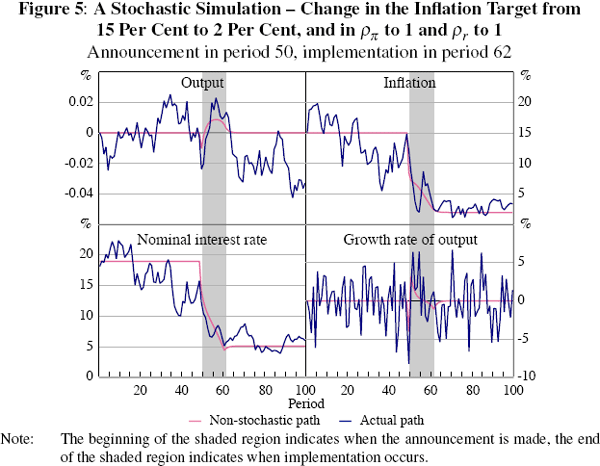
to conduct stochastic simulations. The blue lines in Figure 5 show a stochastic
simulation with the following characteristics: the benchmark parametrisation
with an inflation target of 15 per cent per annum until period 50; at which
time it is announced that in 12 periods time, a lower inflation target of
2 per cent per annum and a more aggressive long-run response to inflation
deviations from that the new target will be in place:  . The different policy
rules give rise to different dynamics, as one would expect. It is interesting
to note, however, that the properties of the new regime seem to be inherited
shortly after the announcement is made.
