RDP 2010-01: Reconciling Microeconomic and Macroeconomic Estimates of Price Stickiness Appendix A: The Model

The economy consists of a unit interval of identical households, N final-goods producers, a continuum of intermediate-goods producers and a monetary authority.

There is a continuum of intermediate-goods producers, indexed on the unit interval (0, 1]. Each sector of the economy is represented by a sub-interval (Ψ_j−1, Ψ_j], where 0 = Ψ₀ <Ψ₁ < ... < Ψ_N = 1. The sub-intervals are not necessarily of the same length, so the measure of sector j is given by γ_j = Ψ_j – Ψ_j−1. A final-goods producer in sector j only uses intermediate goods produced by intermediate-goods firms belonging to the sub-interval (Ψ_j−1, Ψ_j].

A.1 Households

Given initial holdings of bonds, B₋₁, and money, H₋₁, the sequence of wages, prices for final consumption goods, prices for the aggregate consumption good and nominal interest rates and the sequence of monetary transfers and dividends , the sequence of aggregate consumption, consumption of final consumption goods, money holdings, labour supply and bond holdings, solves the following intertemporal maximisation problem

subject to

Using the Lagrange multiplier Λ_t on the budget constraint, we get the following first-order conditions

We also have

We assume the preference process evolves as follows

A.2 Final-goods Firms

There are N sectors, indexed by j. Final-goods firms are perfectly competitive and make zero profits in equilibrium. They sell final goods to households that are produced using inputs from intermediate producers from their sector.

In period t, final-goods firms take as given their total production, and prices for their output and intermediate-goods prices, , and solve the following cost-minimisation problem

subject to

There is also a zero-profit condition that must also be satisfied

The first-order conditions become

where

A.3 Intermediate-goods Firms

Intermediate-goods firms are monopolistically competitive. Intermediate-goods producers in sector j can only change their prices in any given period with Calvo probability θ_j. Once prices have been determined, intermediate-goods firms produce to meet demand for their good from final-goods producers and other intermediate-goods producers. Demand for labour and other intermediate goods are determined by cost minimisation. Firm i in sector j takes wages, W_t , and the price for the aggregate intermediate good, , as given to solve the following cost-minimisation problem

subject to:

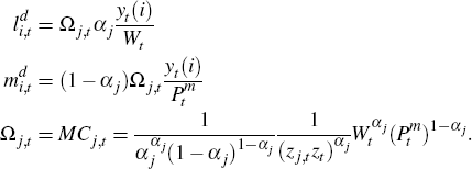
where: z_j,t is sector-specific productivity; z_t is the state of aggregate productivity; is labour demanded by firm i; and is firm i's demand for the aggregate intermediate good. The production constraint is binding and the Lagrange multiplier on the production constraint, Ω_j,t , is the nominal marginal cost and is sector specific. First-order conditions are:

We define:

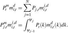
where is the demand for output from sector j by firm k, which can be expressed as follows:

So firms decide how to allocate their expenditure on intermediate goods across sectors, then decide within a sector from which firms it will source its intermediate inputs, given intermediate-goods prices, {P_t(i)}_i∈(0,1], so that

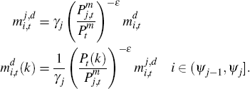
From cost minimisaton, we find that:

Using these results, we can derive the following expressions for the aggregate price index, the sectoral price indices and an expression for a firm's demand for intermediate inputs

When firms are able to reset their prices, they solve the following problem:

First-order conditions give us:

Dividends distributed to households are just period t profits:

and

In equilibrium, total dividends to households will equal nominal value added less total nominal payments to labour ().

We assume that the aggregate technology and sectoral technology processes evolve as follows

where: μ_z is the average growth rate of aggregate technology; ε_z,t is the shock to aggregate technology, and ε_z,j,t is the sector-specific technology shock.

A.4 Monetary Authority

The monetary authority follows the following policy rule:

where and .

Define the gross rate of growth of the money supply to be . Given its target for the nominal interest rate, nominal transfers T_t is given by ( − 1)H_t−1 and is determined endogenously by the money demand equation and money market clearing:

A.5 Market-clearing Conditions

There are N markets for N final goods, a unit interval of markets for intermediate goods, a labour market, a bond market and a money market.

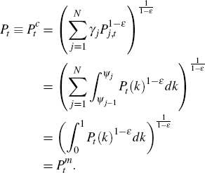
A.5.1 Price indices

We define two price indices. The first, P_t should be familiar to the reader. The second, , is introduced for convenience.

A.5.2 Intermediate goods market-clearing

Using the final goods market-clearing condition:

where:

Since we can use the first-order conditions of the intermediate-goods firm k belonging to sector j to get:

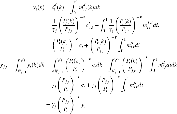
We can also express sectoral output as follows:

where:

So:

A.5.3 Labour market-clearing

Labour demand by each firm is given by

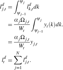
Aggregating this across sector j:

A.5.4 Sectoral price indices

In any given period, a firm in sector j has probability (1 – θ_j) that it can change its price. This implies that the price index for sector j evolves as follows:

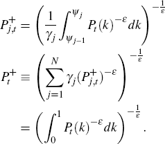
Similarly, for the alternative price index:

A.6 Transformations and Normalisations

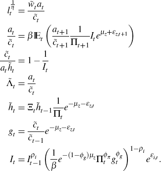
Due to the growth in aggregate technology, we detrend some variables to make them stationary so

We also define:

A.7 Summary of Non-linear Equations

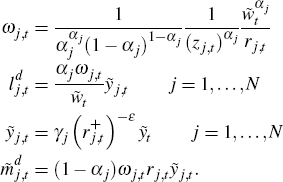
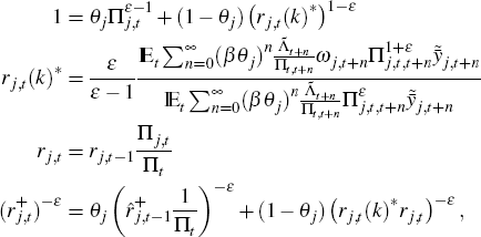
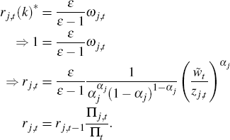
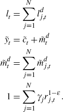
This sub-section summarises the first-order conditions and market-clearing conditions required to solve the model at the sectoral level (rather than at the firm level). For completeness, and the interest of the reader, we present equations for sectors subject to the Calvo mechanism and those with flexible pricing, even though the latter are not used.

For k ∈ (Ψ_j−1, Ψ_j] and j = 1,...,N:

Sticky price sector indices follow

where and .

Flexible price sector prices:

The market-clearing and aggregation equations become:

Stochastic processes are

A.8 Log-linearised Equations

Using the equations above, we denote the log-deviation from trend for variable x to be .

Note that .

Sectoral variables, market-clearing and aggregation equations

where and represent the steady-state shares of value added and intermediate input of gross output.

Flexible prices are set as a constant mark-up over nominal marginal costs while sticky price inflation evolves according to the New-Keynesian Phillips Curve.

Flexible price sectors:

Sticky price sectors:

Driving variables:

In summary, we have 8N + 11 endogenous variables and equations, which completes the model.