RDP 9108: Australia's Real Exchange Rate – Is it Explained by the Terms of Trade or by Real Interest Differentials? 4. Results
September 1991
- Download the Paper 531KB
(a) Unit Root Tests
All series used in the estimation are tested for deterministic and stochastic non-stationarity. The results of these tests are presented in Appendix 1. For many of the series, the results are ambiguous. For some of the series, there is evidence of 2, 1 or 0 unit roots. This lack of clarity is due in part to the small sample period being used.
Our first conclusion is that the real exchange rate has one unit root. This conclusion is based on the fact that, for a majority of the three time periods studied, two of the three tests accept this hypothesis at a 1 per cent level of significance. This result confirms the results of other studies (e.g. Blundell-Wignall and Gregory (1990) and Corbae and Ouliaris (1991)) and accepts the hypothesis that the Australian real exchange rate follows a non-stationary process rather than exhibiting only temporary deviations from purchasing power parity.
By the same criterion, we also find that the terms of trade and long real interest differential series have one unit root.[12]
By contrast, the short real interest differential series with three month expectations (SHORT(B3) and SHORT(F3)) appear to be stationary, that is, they have no unit roots, again looking at all the three different time periods.[13] However, the short real interest differential series with 12 month backward looking expectations (SHORT(B12)) shows much weaker evidence of being stationary than the other two series. Over the post-float period, we tentatively conclude that it has 1 unit root.
Examination of the Tables in Appendix 1 shows the low power of all three tests. Note, in particular, that the G(p,q) test only rejects the null of stationarity in one case.
In this paper we are attempting to explain long run movements in the level of Australia's real exchange rate especially over the period since the float. Since we conclude that this series is non-stationary, its long run behaviour must be explained by other non-stationary series. Hence at this point we exclude the stationary short real interest differential series (SHORT(B3) and SHORT(F3)) from any further analysis. We apply the technique of cointegration to the real exchange rate, terms of trade, long real interest differential and non-stationary short real interest differential (SHORT(B12)) series.
(b) The Real Exchange Rate and the Terms of Trade
Using quarterly data 1970 – 1988, Blundell-Wignall and Gregory (1990) find evidence for a stable long run relationship between the Australian real exchange rate and the terms of trade. Table 2 displays our results. There is mixed evidence for a long run stable relationship between the terms of trade (TOT) and the real exchange rate. For both the long sample period (1969:4 to 1990:4) and the post-float period (1984:1 to 1990:4), the three statistical tests for cointegration give conflicting results. For both samples, the H(p,q) test accepts the null hypothesis of a cointegrating relationship, while the ADF and the Z(t) tests give mixed signals. Thus, the ADF test accepts the null of no cointegration for the long sample, but rejects it (at 10% level of significance) for the post-float period. The Z(t) test rejects the null of no cointegration (at 15% level of significance) for the long sample, but accepts it for the post-float period.
| Explanator | Sample period | Coefficient Estimate | Test Statisticsa | ||||
|---|---|---|---|---|---|---|---|
| E-G | P-Hb | t-statistic | ADF | Z(t) | H(p,q) | ||
| TOT | 69:4–90:4 84:1–90:4 |
0.91 1.06 |
1.08 1.08 |
6.11 4.42 |
−2.13 −3.07** |
−2.89* −2.61 |
6.30 7.84 |
| TOT(C) | 84:1–90:4 | 0.82 | 0.92 | 3.02 | −2.26 | −2.57 | 8.03 |
| LONG | 69:4–90:4 84:1–90:4 |
−0.016 0.045 |
−0.029 0.056 |
−1.84 3.74 |
−2.00 −3.39*** |
−2.15 −3.52*** |
5.02 7.29 |
| SHORT (B12) | 69:4–90:4 84:1–90:4 |
−0.017 0.015 |
−0.029 0.020 |
4.63 1.07 |
−2.16 −2.09 |
−2.45 −2.51 |
4.35 6.67 |
a. All of these statistics are based on regressions containing a
constant but no time trend. The ADF and Z(t) statistics are based on the E-G
regressions, while the H(p,q) statistics are based on the P-H regressions. For the
ADF and the Z(t) tests, the null hypothesis is no cointegration. If
the test statistic is more negative than the critical value then
the null is rejected, i.e. cointegration is accepted. 5%, 10% and 15% critical
values for these test statistics are: −3.37, −3.07, and −2.86
(Phillips and Ouliaris (1990)). For the H(p,q) statistic the null hypothesis is
cointegration. Under this null, this statistic is asymptotically
distributed as a chi-squared with q-p degrees of freedom. We use p = 0, q = 5. 5%,
10% and 15% critical values for this test statistic are: 11.07, 9.24 and 8.12. |
|||||||
Interestingly, in the post-float period, two of the three tests (the ADF and Z(t) tests) find that the real exchange rate is not cointegrated with TOT(C) – the terms of trade measured by the ratio of commodity prices to import prices. This finding is surprising as most of the movement in export prices comes from changes in commodity prices, and thus there is a general expectation that the real exchange rate is primarily determined by commodity prices.
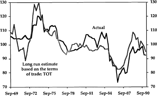
Blundell-Wignall and Gregory estimate that, in response to a 1% change in the terms of trade, the real exchange rate changes by about 0.63% pre-float, by about 1.4% post-float, and by about 1.05% for their full sample. By contrast, using a somewhat longer run of data, our estimated relationships are almost the same in the post-float period as in the whole sample. For a 1% change in the terms of trade, we estimate a change in the real exchange rate of between 0.82% and 1.08%. Graph 4 shows the level of the real exchange rate over the whole sample period and the long run estimate of the real exchange rate derived from the Phillips-Hansen estimated cointegrating relationship with the terms of trade (TOT).[14]

(c) The Real Exchange Rate and Real Interest Differentials
Meese and Rogoff (1988) examine several bilateral real exchange rates with the US to determine whether there is a long run stable relationship with the respective real interest differentials. They find that their short real interest differentials are stationary, and although their long real interest differentials and real exchange rate series are both non-stationary, there is no stable long run relationship between them.
Table 2 (above) contains coefficient estimates and cointegration tests for the relationship between the Australian real exchange rate and real interest differentials. As the Table shows, over the full sample period there is no strong evidence that the real exchange rate is cointegrated with either real interest rate differential, and the coefficient estimates on the interest differentials are of the wrong sign. After the float, there continues to be no strong evidence of cointegration with the short real interest differential. By contrast, there is very strong evidence of cointegration between the real exchange rate and the long real interest rate differential – with all three tests accepting cointegration at a 5% level of significance. Both the Engle-Granger and Phillips-Hansen methods give coefficient estimates on the long real interest differential of about 0.05. Because the real interest differentials are entered in levels and the real exchange rate in logs, these results imply that a 1 percentage point increase in the long real interest differential is associated with an average appreciation of the real exchange rate of about 5 per cent.
(d) Do the Terms of Trade and Real Interest Differentials Jointly Explain the Real Exchange Rate?
We have established that there is some evidence after the float of a stable relationship between the real exchange rate and the terms of trade and strong evidence of a stable relationship between the real exchange rate and long real interest differentials. In this sub-section, we extend our analysis in three ways. Firstly, we examine both monthly[15] and quarterly data. Secondly, we extend our analysis to examine cointegrating relationships between all three variables. Finally, we use the Johansen (1988) procedure to examine the number of cointegrating relationships between the three series.
Tables 3 and 4 present the results from estimation on a quarterly and on a monthly basis respectively.
| SINGLE EQUATION ESTIMATES | JOHANSENb | ||||||||||||
|---|---|---|---|---|---|---|---|---|---|---|---|---|---|
| Coefficient Estimatesc |
Test Statisticsd |
Coefficient Estimates |
Tests for the number of cointegrating relationships | ||||||||||
| E-G | P-H | t-statistic | ADF | Z(t) | H(p,q) | 1st Vector | 2nd Vector | Lambda Max 5% (10%) |
Trace 5% (10%) |
||||
| TOT LONG | 0.95 0.007 | 0.97 0.004 | 2.73 0.21 | −3.40* |
−2.82 |
7.32 |
1.30 0.04 | −0.41 0.06 | 0(3) |
3(3) |
|||
| TOT(C) LONG | 0.43 0.029 | 0.43 0.031 | 1.21 1.66 | −3.42* |
−3.39* |
8.37* |
−1.42 0.20 | 3.39 −0.14 | 2(3) |
2(3) |
|||
| TOT SHORT (B12) | 1.23 −0.014 |
1.24 −0.019 |
6.26 −2.20 |
|
−2.02 |
−2.08 |
5.84 |
|
1.32 −0.003 |
1.01 −0.037 |
2(2) |
2(2) |
|
| TOT(C) SHORT (B12) | 0.84 −0.003 |
0.95 −0.010 |
3.11 −0.75 |
|
−2.09 |
−2.47 |
5.99 |
0.49 0.047 |
2.57 −0.119 |
3(3) |
3(3) |
||
a. In this Table and in Table 4, the relationships between the real
exchange rate and its determinants are estimated using three methods. In the first
part of the Table are the single equation estimates – based on the
Engle-Granger (E-G) and Phillips-Hansen (P-H) approaches. In the second part of the
Table are the Johansen estimates – based on the estimation of the full system
of equations. |
|||||||||||||
| SINGLE EQUATION ESTIMATES | JOHANSEN | ||||||||||||
|---|---|---|---|---|---|---|---|---|---|---|---|---|---|
| Coefficient Estimates |
Test Statistics |
Coefficient Estimates |
Tests for the number of cointegrating relationships |
||||||||||
| E-G | P-H | t-statistic | ADF | Z(t) | H(p,q) | 1st Vector | 2nd Vector | Lambda Max 5% (10%) |
Trace 5% (10%) |
||||
| TOTM(I) | 0.93 | 0.94 | 8.67 | −2.46 | −4.22*** | 9.75** | |||||||
| TOTM(C) | 0.74 | 0.85 | 6.29 | −1.85 | −3.91*** | 14.61*** | |||||||
| TOTM(X) | 0.78 | 0.82 | 7.73 | −2.69 | −4.54*** | 13.79*** | |||||||
| LONGM | 0.040 | 0.054 | 5.98 | −2.77 | −3.45*** | 2.60 | |||||||
| SHORTM(B12) | 0.025 | 0.038 | 3.25 | −1.53 | −3.30** | 6.20 | |||||||
| TOTM(I) LONGM | 0.86 0.004 | 0.70 0.015 | 4.27 1.79 | −2.59 |
−4.20*** |
7.21 |
0.21 0.042 | 1.59 −0.014 | 2(2) |
2(2) |
|||
| TOTM(C) LONGM | 0.43 0.023 | 0.35 0.033 | 2.43 4.22 | −2.67 |
−3.90*** |
14.43*** |
0.30 0.048 | 0.14 0.030 | 3(3) |
3(3) |
|||
| TOTM(X) LONGM | 0.62 0.013 | 0.51 0.024 | 3.79 3.02 | −2.96 |
−4.39*** |
10.02** |
0.34 0.033 | 1.26 −0.002 | 1(2) |
1(2) |
|||
| TOTM(I) SHORTM(B12) | 0.91 0.001 | 0.90 0.002 | 6.91 0.41 | −2.50 |
−4.23*** |
9.93** |
0.49 0.048 | 3.55 −0.178 | 2(2) |
2(2) |
|||
| TOTM(C) SHORTM(B12) | 0.63 0.011 | 0.68 0.014 | 4.86 2.04 | −2.28 |
−4.07*** |
16.52*** |
0.12 0.068 | 2.16 −0.063 | 3(3) |
3(3) |
|||
| TOTM(X) SHORTM(B12) | 0.72 0.006 | 0.71 0.009 | 6.30 1.55 | −2.93 |
−4.63*** |
12.63*** |
0.05 0.069 | 0.91 −0.019 | 3(3) |
3(3) |
|||
| For an explanation of this Table see the notes to Table 3. | |||||||||||||
Test statistics using quarterly data again show much stronger evidence of cointegration when long real interest differentials are included in the relationship than when short ones are (Table 3). The evidence is strongest using TOT(C) and LONG as regressors. In this case, both the ADF and Z(t) tests reject the null of no cointegration at a 15% level of significance, while the H(p,q) test accepts the null of cointegration at a 10% level.[16] Coefficient estimates on both the terms of trade and long real interest differentials are lower than the independent estimates given in Table 2. This reflects the fact, highlighted in Table 1, that the terms of trade and the long real interest differential are highly positively correlated after the float.
Using the Johansen procedure to analyse the same data gives mixed evidence. Anywhere between 0 and 3 cointegrating relationships are identified. The existence of three cointegrating relationships implies that each series in the estimation is stationary. With the possible exception of SHORTM(B12), we have already established to our satisfaction that this is not the case. However, there may be more than one cointegrating relationship. We discuss this case later in this section.
Before doing that, we report results of monthly estimation after the float in Table 4. The evidence for a stable long run relationship between the real exchange rate and a single other variable is again stronger with the long real interest differential than with the short real differential, or with any of the measures of the terms of trade. Note that, in all the regressions which use a single explanatory variable (i.e. the first five), the explanatory variable is of the expected sign and highly significant (judged by the t-statistics on the Phillips-Hansen regressions). The coefficient estimates in these regressions are very similar to those estimated on quarterly data after the float (Table 2).
The results of single equation estimation when both the terms of trade and real interest differentials are used as explanatory variables are reported as the last six regressions in Table 4. The evidence in favour of a stable long run relationship is mixed – though it is again more favourable with long rather than short real interest differentials. The coefficient estimates are always of the expected sign.[17] With the exception of two of the regressions with the short real differential, both explanatory variables in the Phillips-Hansen regressions are highly significant.
Applying the Johansen technique to these data once again gives mixed results. Anywhere between 1 and 3 cointegrating relationships are identified. As before, we do not further analyse the case when three cointegrating relationships are identified (e.g. using TOTM(C) and LONGM as explanators). We recognise that these results contradict our original analysis of the data and are another indication of the low power of the time series tests in short runs of data.
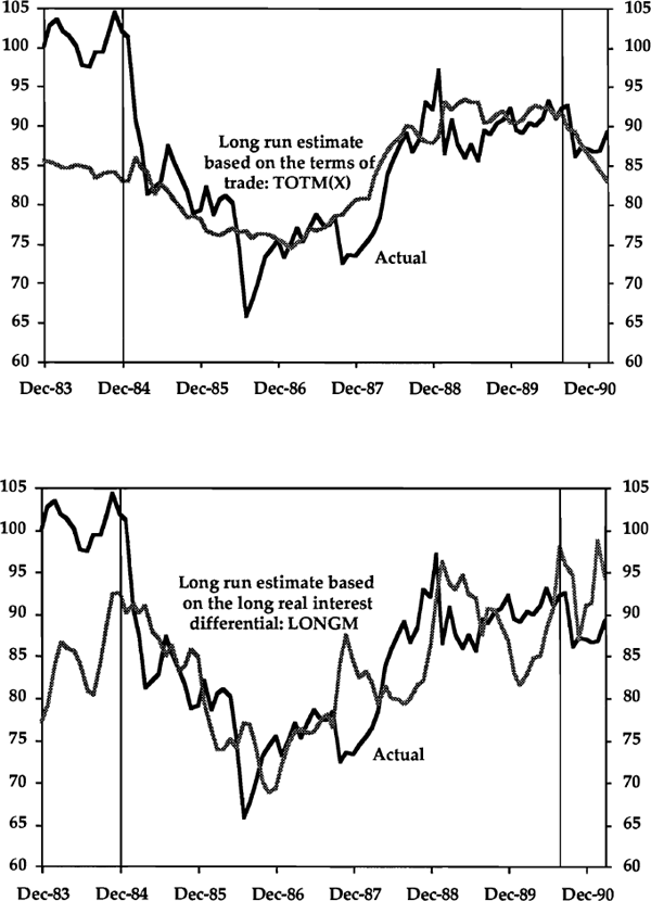
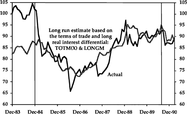
Both panels of Graph 5 show the level of the monthly real exchange rate series (RERM) from December 1983 to March 1991 (i.e. since the float of the $A). The upper panel also shows the long run real exchange rate derived from the Phillips-Hansen estimated cointegrating relationship (P-H ECR) with the terms of trade (TOTM(X)), while the lower panel shows the long run real exchange rate derived from the P-H ECR with the long real interest differential (LONGM). Graph 6 shows the level of the monthly real exchange rate as well as the long run real exchange rate derived from the P-H ECR with both the terms of trade (TOTM(X)) and the long real interest differential (LONGM). The three cointegrating regressions used for Graphs 5 and 6 are reported in Table 4. Note that they are all estimated for the period 1984:12 to 1990:9, i.e. the period between the vertical lines on the graphs.


The cointegrating relationship used for Graph 6 is chosen because of its appealing properties. At a 5% level of significance, the Z(t) statistic rejects the null of no cointegration, the H(p,q) test accepts the null of cointegration and both tests from the Johansen method accept the hypothesis of a single cointegrating relationship between these two variables and the real exchange rate.[18] Finally, the t-statistics for the regression imply that both variables are highly significant.
Interestingly, in Graph 6, the eight months after October 1987 stand out as the longest time in the estimation period during which the real exchange rate deviates in one direction from its long run estimate. An obvious reason for this behaviour of the exchange rate was the world stockmarket crash. At the time, this was widely expected to lead to a world-wide recession and hence a fall in commodity prices. In fact, the event preceded a world-wide boom in 1988.
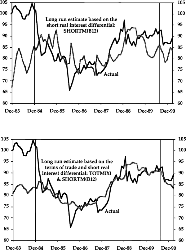
For completeness, Graph 7 shows two Phillips-Hansen estimated cointegrating relationships using SHORTM(B12). Note that the evidence from Table 4 suggests that the relationship shown in the bottom panel of Graph 7 is not a stable long run relationship.

We now briefly discuss the out-of-sample behaviour of the estimated relationships used for Graphs 5, 6 and 7. For the year 1983:12 to 1984:11 (before the estimation period), all the estimated long run real exchange rate series very substantially underestimate the actual real exchange rate.
Interestingly, they share this property with the cointegrating relationship estimated between the terms of trade and the real exchange rate for the period 1969 to 1990 and shown in Graph 4. Thus, during the first year after the float, all our evidence suggests that the Australian real exchange rate was well above the level consistent with either the terms of trade or the relative level of real interest rates.
In the six months 1990:10 to 1991:3 (after the estimation period), it appears that the cointegrating relationship based on both the terms of trade and the long real interest differential has performed better than either of the relationships using a single explanator (compare Graph 6 with Graph 5) or than the relationships estimated with the short real differential (Graph 7).
There are five sets of variables from Tables 3 and 4 for which the Johansen method suggests that there may be two cointegrating relationships. In these cases, interpretation is not straightforward because the estimated cointegrating relationships are not unique – any linear combination of two cointegrating vectors also represents a cointegrating relationship (see footnote 6). One way to interpret the results is to transform the vectors to relationships involving only one of the explanators. In this way, the coefficient estimates can be compared with the independently derived single equation estimates presented in Tables 2 and 4. For these five cases, the original Johansen coefficient estimates and the transformed estimates are reported in Table 5. It is encouraging that, with one exception, the transformed coefficient estimates are all of the expected sign. They are of the same order of magnitude as the single equation estimates from Tables 2 and 4 (although, in all cases, the transformed estimates of the terms of trade are larger).
| Explanators | Original Estimates | Transformed Coefficient Estimates | ||
|---|---|---|---|---|
| First Vector | Second Vector | First Vector | Second Vector | |
| Quarterly 84:1 – 90:4 | ||||
| TOT(C) | −1.42 | 3.39 | 1.41 | 0.00 |
| LONG | 0.20 | −0.14 | 0.00 | 0.099 |
| TOT | 1.32 | 1.01 | 1.35 | 0.00 |
| SHORT(B12) | −0.003 | −0.037 | 0.00 | −0.148 |
| Monthly 84:12 – 90:9 | ||||
| TOTM(I) | 0.21 | 1.59 | 1.25 | 0.00 |
| LONGM | 0.042 | −0.014 | 0.00 | 0.051 |
| TOTM(X) | 0.34 | 1.26 | 1.21 | 0.00 |
| LONGM | 0.033 | −0.002 | 0.00 | 0.046 |
| TOTM(I) | 0.49 | 3.55 | 1.14 | 0.00 |
| SHORTM(B12) | 0.048 | −0.178 | 0.00 | 0.084 |
Footnotes
In a world with deregulated financial flows, it is hard to understand why either short or long real interest differentials could be non-stationary. This issue is addressed in the Discussion section. [12]
This statistical evidence – that real short-term interest differentials seem to be stationary – is consistent with the findings of Meese and Rogoff (1988). It is also consistent with the work of Campbell and Clarida (1987) and Tarditi and Menzies (1991) who examine the relationship between the level of real short-term interest differentials and the log level of the real exchange rate. Both of these studies find this relationship to be insignificant. [13]
The real exchange rate presumably responds more to terms of trade changes which are perceived to be permanent than to those perceived to be transitory. Our approach does not take this distinction into account. [14]
Both graphical and econometric evidence suggest that the relationship between the variables is not stable for several months after the float. As a consequence, our monthly analysis is from 1984:12 to 1990:9. [15]
Note, however, that two of the three test statistics show stronger evidence of cointegration with LONG as the sole explanator, than with both LONG and TOT(C) as explanators (see Tables 2 and 3). [16]
Since our real interest differentials are expressed as percent per annum, the theoretical restriction on α, the coefficient on the real interest differential in equation (2), is α > 0.01. Based on the P-H estimates post-float, this restriction is accepted in all but one equation where long real interest differentials are used as an explanator (the exception is the first regression in Table 3). However, the restriction is accepted only in one case where short real interest differentials are used along with a terms of trade explanator. With time measured in years, the implied speed of adjustment parameter is in the range 0.5 ≤ θ ≤ 0.8. This is comparable to the Meese and Rogoff (1988) and Campbell and Clarida (1987) results. [17]
Unfortunately, the ADF statistic accepts the null of no cointegration, but you can't have everything. [18]