RDP 2000-05: A Small Model of the Australian Macroeconomy 2. Overview

We begin the overview by discussing some of the model's characteristics, before turning to a few stylised facts about the Australian macroeconomy over the past fifteen years that provide motivation for the specification of some of the model equations. We then discuss the structure of the model in more detail.

2.1 Characteristics

Three features broadly characterise the model. It is empirical, aggregate and non-monetary. We briefly address each of these in turn.

Macroeconomic models vary along a spectrum ranging from empirically based models to those primarily or exclusively derived from theoretical, microeconomic principles. This spectrum exists because experience has revealed an undesirable trade-off between the extent to which a macroeconomic model is based on theoretical, microeconomic principles and its capacity to fit the economic data.^[1]

The model in this paper is predominantly empirically based. The model equations are estimated econometrically. Restrictions on sets of estimated coefficients in the three price equations are imposed in order to generate steady-state properties that accord with our theoretical priors.

There are both backward- and forward-looking inflation expectations in the model. Real interest rates, which appear in the equations for output and the real exchange rate, are calculated using past inflation to deflate nominal interest rates. In the equation for unit labour costs, there are both backward- and forward-looking expectations, with the latter derived from the bond market. Rational model-consistent expectations do not, however, play a role in the model.

The model is highly aggregated, which is necessary to keep it as small as it is. Perhaps the most obvious example of this is that output is modelled in a single equation. In this respect, the model more closely resembles a small vector auto-regression model than a larger scale macroeconomic model in which the major expenditure components and sectors of the economy are treated separately. The model is, however, larger than most small vector auto-regression models in that, as well as the five endogenous variables explained by the model, there are a further ten exogenous variables that appear in one or more of the model equations.

Finally, the model is non-monetary – that is, there is no explicit role for monetary quantities. As in most countries, the stable relationship between money and nominal output broke down in Australia in the 1980s. By the early 1990s, a stable long-run relationship between money, income and interest rates had become hard to find (de Brouwer, Ng and Subbaraman 1993) and since then researchers have come to assign money little or no causal role in the transmission mechanism of monetary policy. Reflecting this, more recent work on the transmission of monetary policy to output has used the real interest rate to measure the stance of monetary policy (for example, Gruen, Romalis and Chandra (1997)). Furthermore, neither the inflation equation derived in de Brouwer and Ericsson (1995), nor the simultaneous system of wages and prices in Cockerell and Russell (1995) contain money.

The characterisation of the model as empirical, aggregate and non-monetary stands it apart from many other macro-econometric models, both for Australia, and for other countries. Nevertheless, it provides a useful framework within which to forecast the evolution of the Australian economy and conduct policy simulations over the short to medium run.

2.2 Stylised Facts About the Australian Macroeconomy

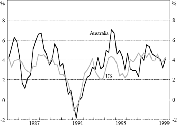
One of the best-documented stylised facts about the Australian business cycle is its close relationship with the US business cycle, as shown in Figure 1. There have been several suggestions for the strength of this relationship. In the shorter run, links between financial markets (Gruen and Shuetrim 1994; de Roos and Russell 1996; and Kortian and O'Regan 1996), effects on Australian business confidence (Debelle and Preston 1995), and a disproportionate response of Australian exports to the US business cycle (de Roos and Russell 1996) all play a role. In the longer run, technology transfer from the US seems to be important (de Brouwer and Romalis 1996). The strong relationship between the Australian and US business cycles forms the basis for the equation for non-farm output in the model.

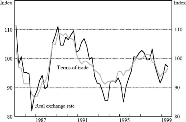
A second stylised fact about the macroeconomy is the strong relationship between the Australian trade-weighted real exchange rate and the terms of trade for goods and services, shown in Figure 2. With roughly three-fifths of exports accounted for by commodities, Australia's terms of trade are volatile. The close co-movement of the terms of trade and the real exchange rate remains something of a puzzle, however (Gruen and Kortian 1996). For reasons that remain unclear, the two series are much more correlated than for other advanced commodity exporting countries like Canada or New Zealand. Not surprisingly, this close relationship, particularly since the float of the Australian dollar in 1983, has formed the basis of econometric models of the Australian exchange rate for many years (see, for example, Blundell-Wignall and Gregory (1990), Gruen and Wilkinson (1991), and Tarditi (1996)). This relationship also forms the basis for the real exchange rate equation in the model described here.

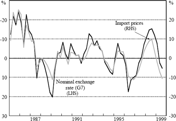
Movements in the exchange rate have important implications for the domestic-currency price of imports, and hence, for consumer price inflation. Import prices affect consumer prices directly, since a proportion of the consumption basket is imported, as well as via imported intermediate and capital goods. Most of the movement in import prices is attributable to fluctuations in the exchange rate, and pass-through of exchange rate movements to import prices is rapid (Figure 3). The pass-through of exchange rate changes to import prices forms the basis of the import price equation in the model.

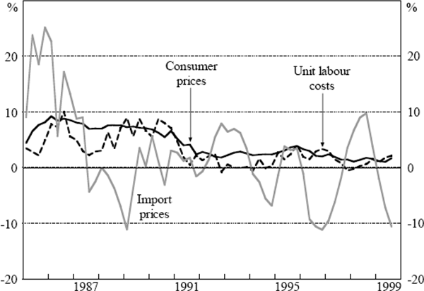
Consumer price changes, although influenced by import price movements, are dominated by changes in domestic unit labour costs. When nominal wages growth exceeds the growth of labour productivity, firms' margins are squeezed leading to upward pressure on prices. Figure 4 shows the fairly close relationship between growth in consumer prices and unit labour costs. At times, however, when import prices are rising or falling rapidly, their influence on consumer prices is also evident. Thus, for example, import prices were putting upward pressure on consumer price inflation in 1985, and downward pressure in 1996/97. The relationship between unit labour costs, import prices and consumer prices forms the basis of the consumer price equation in the model.

2.3 Structure

As previously mentioned, there are five endogenous and ten exogenous variables in the model. The relationships between these variables are summarised in the flow chart in Figure 5, with the endogenous variables shown in bold type.

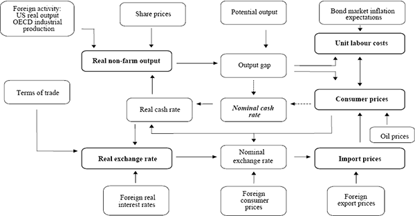
We can use the flow chart to draw out the main linkages in the model. The effect of monetary policy on the economy is modelled in terms of the effect that changes in the policy interest rate, the nominal cash rate, have on the real cash rate. The real cash rate in turn has a direct impact on real output and the real exchange rate, with a higher real cash rate reducing output growth for a time, and appreciating the real exchange rate.

The real exchange rate is determined by the terms of trade and the differential between domestic and foreign real interest rates.

Non-farm output growth in the model is determined predominantly by foreign activity (US real output and OECD industrial production) and by lags of the domestic real interest rate. The level of share prices also plays a role. Australian output growth in the model's steady state is proportional to the assumed rate of steady-state output growth in the US. This relationship, which is quite strong in the data, can presumably be explained as a consequence of technological transfer and catch-up. Domestic output in the steady state is, however, independent of the rate of domestic consumer price inflation, a standard result for macroeconomic models that focus on the short to medium run.

The supply potential of the domestic economy is not modelled explicitly. Potential output is estimated by smoothing actual output, and adjusting the resultant series so that consumer price and unit labour cost inflation are steady when output is at potential. Potential output is also constrained to equal actual output in the steady state of the model.

The difference between actual and potential output, the output gap, has a direct influence on both unit labour cost and consumer price inflation. Changes in this gap also have an influence, so that there is upward pressure on consumer prices when output is growing faster than potential, and downward pressure when it is growing slower than potential.

Unit labour costs are influenced not only by the output gap but also by past consumer price inflation, as well as by forward-looking inflation expectations which in the model are derived from the bond market. The unit labour cost equation exhibits a vertical long-run Phillips curve in the steady state, again a standard result for macroeconomic models. Imposing this vertical long-run Phillips curve in a way that is accepted by the data is not, however, a straightforward exercise – it involves splitting the sample into two parts and imposing it only on the latter part (see Section 3.4).

Consumer prices are modelled as a mark-up on unit labour costs and import prices, with the margin between price and input costs varying cyclically with the output gap, and also depending in the short run on the domestic price of oil. Consumer prices in the steady state are, up to a constant, a linear combination of unit labour costs and import prices with weights that sum to one – that is, the equation exhibits static homogeneity.^[2]

Import prices are determined jointly by foreign export prices and the nominal exchange rate, with changes in the exchange rate passing through rapidly to import prices. Traded goods prices satisfy purchasing power parity (up to a constant) in the steady state.

The dotted lines in the flow chart signify the presumed link from current (and expected future) outcomes for consumer prices and the output gap to the policy interest rate, the nominal cash rate. As the model is described in the paper, this link is not formalised. It is straightforward, however, to augment the model with a policy reaction function, such as a Taylor rule, or something more sophisticated.

Footnotes

Two examples give a flavour of this trade-off. Firstly, the joint hypothesis of uncovered interest parity and rational expectations in the foreign exchange market has impeccable theoretical credentials, but is usually rejected by the data, for reasons that have thus far defied explanation in terms of economic theory (Engel 1995). Secondly, small macroeconomic models based explicitly on optimising behaviour by representative economic agents provide a worse fit to the economic data, and appear less robust to the Lucas critique, than models that assume backward-looking adaptive behaviour on the part of economic agents (Estrella and Fuhrer 1998, 1999). [1]

Our theoretical priors would also lead us to expect that the consumer price equation would exhibit dynamic homogeneity, so that steady-state changes in the rate of inflation, that are shared by unit labour costs, import prices, oil prices and consumer prices, would have no real effects. This property is, however, overwhelmingly rejected by the data and is not imposed. The import price equation also fails to exhibit dynamic homogeneity. The implications of these rejections are discussed later. [2]