RDP 2000-05: A Small Model of the Australian Macroeconomy 5. Simulations

Having specified the model and characterised its steady state, we can now turn to its uses. The model can be used to generate forecasts of the endogenous variables, based on assumptions about the future behaviour of the exogenous variables. It can also be used to explore the linkages between the dynamics of the macroeconomy and the appropriate setting of monetary policy. To do so involves augmenting the model with a policy reaction function, such as a Taylor rule, or an objective function for policy. A number of papers have addressed these issues using earlier versions of this model (de Brouwer and O'Regan 1997; Lowe and Ellis 1997; Shuetrim and Thompson 1999).

Rather than updating this work here, we simply illustrate the model's properties with several dynamic simulations. We track the response of the model to five events: a permanent one percentage point increase in the real cash rate, and one-off one per cent shocks to the level of output, import prices, unit labour costs and consumer prices. The real cash rate is held constant throughout the simulations involving one-off shocks. Inflation expectations, , are set equal to the previous period's four-quarter-ended inflation, p_t−1 − p_t−5. We also assume that share prices are unaffected by any of the shocks or by changes to monetary policy.^[13]

All the simulation results report deviations from the steady state. Impulse response functions and 90 per cent confidence intervals, derived using a Monte Carlo procedure, are shown in the graphs.^[14]

5.1 A Permanent Increase in the Real Cash Rate

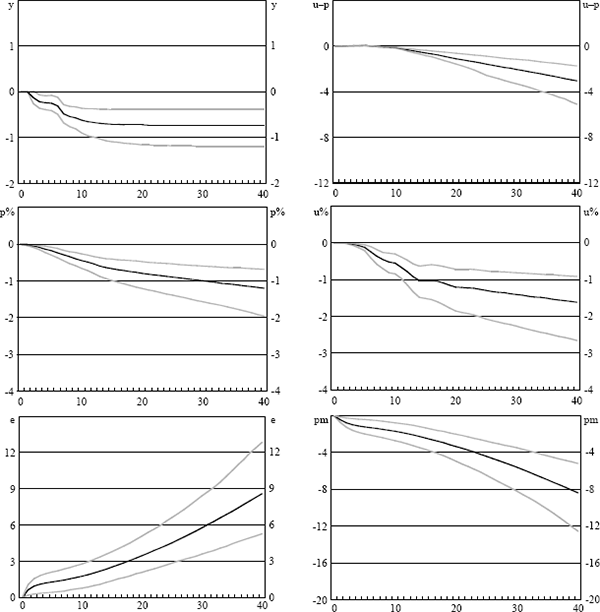
As expected, the tightening of monetary policy has a contractionary effect on the economy. The level of output falls by 0.8 per cent in the long run, with the bulk of this adjustment complete after three years (see Figure 8).

The opening up of a permanent output gap leads to a deflationary cost/price spiral. Annual inflation is reduced by ½ per cent between quarters six and ten and continues to decline indefinitely. The real exchange rate appreciates to a new long-run level in response to higher domestic real interest rates (not shown), while the nominal exchange rate continues to appreciate as domestic prices fall relative to those abroad. Accordingly, import prices decline. Real unit labour costs gradually fall as the trend rate of inflation declines, which illustrates an aspect of the model's lack of neutrality with respect to changes in the inflation rate.

This simulation is, of course, unrealistic in many respects. For one thing, monetary policy would not be expected to have a permanent influence on the domestic real interest rate. For another, the Lucas critique would seem to be particularly relevant to a situation in which the inflation rate was continuously falling (or rising). Economic agents in such a situation would presumably come to anticipate further such changes rather than simply responding to them in an adaptive way. Despite the lack of realism, however, it is of interest to show the cost/price spiral that results from an extended period during which output is kept below potential.

5.2 A One-off Shock to Output

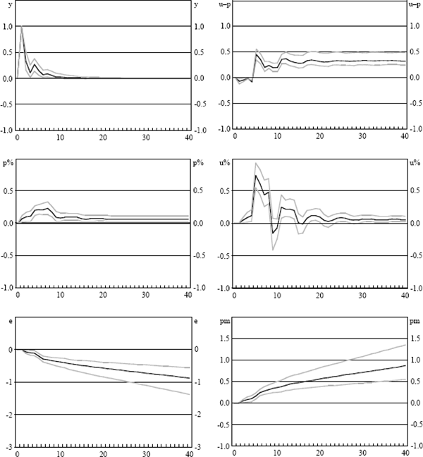
Following a one-off shock, output remains above potential for several quarters while the shock slowly dissipates (see Figure 9). The temporarily higher level of output generates inflationary pressures, and leads to a higher ongoing rate of price and unit labour cost inflation. The level of real unit labour costs rises permanently. Rising domestic consumer prices generate continued nominal depreciation of the exchange rate, but the real exchange rate is unaffected by the shock to output.

5.3 A One-off Shock to Import Prices

A one-off one per cent shock to import prices has a limited effect on the model (not shown). The shock leads to a permanent rise in the levels of consumer prices and unit labour costs, but to only temporary increases in their rates of inflation. The increase in the level of consumer prices prompts an equivalent depreciation of the nominal exchange rate. Since real interest rates are kept constant by assumption, neither output nor the real exchange rate are affected by the shock.

5.4 A One-off Shock to Unit Labour Costs

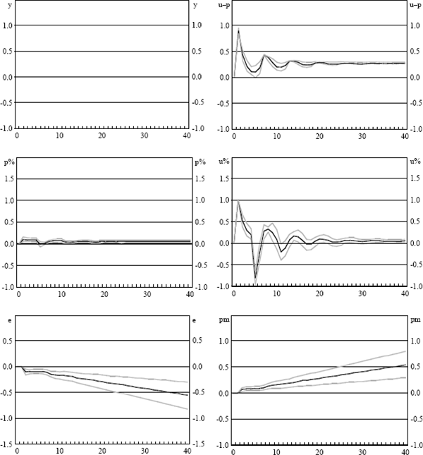
A one-off one per cent shock to unit labour costs permanently raises the rate of unit labour cost and consumer price inflation (see Figure 10). As with other shocks that raise the steady-state rate of inflation, there is a permanent rise in the level of real unit labour costs. Output and the real exchange rate are, however, unaffected by the shock. Reflecting the permanently higher rate of inflation, there is a persistent depreciation of the nominal exchange rate, and a permanently higher rate of import price growth.

The one-off shock to unit labour costs generates oscillations around the new steady state which take several years to dissipate. This is also true of one-off shocks to consumer prices (see below). It seems implausible, however, that such shocks would have such long-lasting impacts on the economy. This feature of the model arises from the estimated dynamics in the unit labour cost equation. From a more fundamental perspective, it may be a consequence of the purely backward-looking inflation expectations that underlie these simulations (see Fuhrer 1997). If so, including a modest amount of forward-looking behaviour into the simulations might alleviate this problem. We leave this possibility as a topic for future research.

5.5 A One-off Shock to Consumer Prices

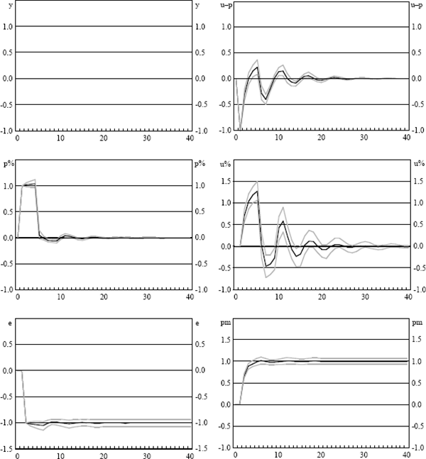
A one-off shock to consumer prices generates a temporary change to the rate of consumer price and unit labour cost inflation (see Figure 11).^[15] As a consequence, no real variables in the system are permanently changed. Inflation returns to its pre-shock rate after about a year, while unit labour cost growth takes longer to adjust and oscillates around its steady state, as discussed above. The level of unit labour costs adjusts to match the shock to prices, preserving the level of real unit labour costs in the model. There is a one-off depreciation of the nominal exchange rate, and a corresponding rise in the level of import prices. Import price growth returns to zero after about a year.

Footnotes

These assumptions are made for simplicity since they render the model entirely backward-looking, and therefore stable with respect to shocks away from the steady state. It would of course be possible to model inflation expectations and share prices in alternative ways. [13]

In the Monte Carlo procedure, residuals are drawn from independent normal distributions with standard deviations equal to those of the residuals from the estimated equations. The point estimates shown are median outcomes from these simulations and differ slightly from OLS results. [14]

This should be contrasted with the result from the previous unit-labour-cost shock, which led to a permanent change to the rate of inflation. From a purely technical perspective, this qualitatively different response to seemingly similar shocks is a consequence of different specifications in the two equations, with a long-run levels relationship present in the consumer price equation but absent from the unit labour cost equation. [15]