RDP 2002-06: Output Gaps in Real Time: are they Reliable Enough to use for Monetary Policy? Appendix B: Statistical Properties of the Phillips Curve Approach

In this appendix we examine the statistical properties of our preferred approach to simultaneously estimating the output gap and the coefficients of our chosen Phillips curve equation. The usual OLS standard errors do not apply because the potential output series is constructed as part of the estimation procedure.

We use a bootstrapping approach to construct multiple sets of ‘pseudo data’ for inflation, and then generate distributions for the estimated values of the parameters in equation (A1), and for the potential output and output gap series, by applying our iterative procedure to each pseudo data set.

Details of the Bootstrapping Procedure

The approach we use, described for the case of our 2001:Q4-optimised Phillips curve equation (see Table 2), is as follows.

Step 1: First, we take the potential output series , parameter estimates , and set of inflation residuals , obtained from iterative estimation of equation (A1) using the actual inflation data.

Step 2: We then generate 1,000 alternative sets of pseudo data for inflation residuals, , each set obtained by making 163 random draws with replacement from the set of initial inflation residuals .

Step 3: For each i = 1, … , 1,000 we then generate a corresponding set of pseudo data for inflation by using equation (A1) – with the for , with the for {γ, δ_i, κ_j, β_j, η_j, ξ_j}, but with the rather than the for {ε_t} – to successively generate new pseudo data from 1961:Q2 onwards. In applying equation (A1) we use the actual data for other variables, as well as for the pre-1961:Q2 data for inflation.

Step 4: For each of these 1,000 sets of pseudo data for inflation we then re-run our iterative procedure for estimating equation (A1), thereby obtaining for each a corresponding alternative potential output series ; alternative set of parameter estimates ; and alternative set of estimated inflation residuals . We can then study the resulting distributions obtained from these 1,000 simulations for each parameter value and for the series.

For reasons discussed in Section 4, it is also of interest to examine Monte Carlo simulations where only the more limited set of (say) post-1976 residuals are used, rather than the full set of residuals.

Results of the Monte Carlo Simulations

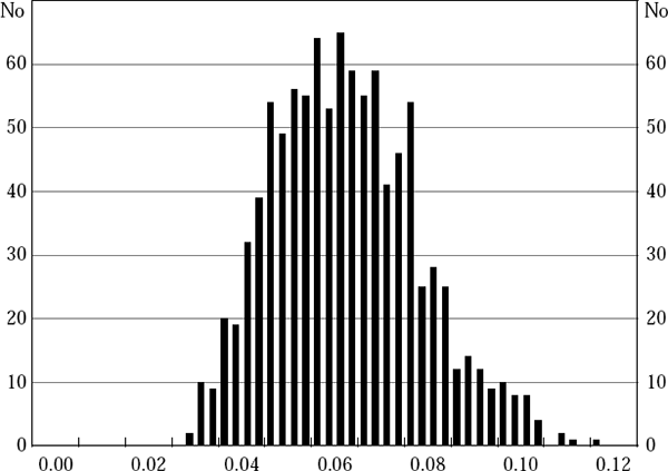
Results from these simulations are shown in Figures 15 and 16 in Section 4 and Figure B1 below.

To assess the statistical significance of our estimates of γ, we also generate 1,000 sets of pseudo data for the final-vintage Phillips curve specification (see Table 2) assuming γ = 0. In 297 cases, the procedure does not converge after 200 iterations, which is perhaps not surprising since a true value of zero for γ implies that the potential output series is indeterminate. For the remaining 703 cases, the t-statistic on γ is always less than the 6.081 reported in Table 2. Given convergence and the high t-statistic, we conclude that the estimate of γ reported in Table 2 is highly statistically significant.

Note that these results are for our final Phillips curve equation. Similar tests were carried out for a selection of other data vintages, with their corresponding Phillips curve specifications, and the same general conclusions were found to hold.^[24]

Footnote

For some early vintages, the iterative procedure fails to converge in some of the Monte Carlo simulations even when the estimated value of γ is used. This is especially true of vintages from around the mid 1970s. This reflects both the short length of these early data vintages (which makes equation estimation more difficult), and the higher fraction of these smaller data sets consisting of data from the period of relative economic turmoil in the first half of the 1970s. [24]