RDP 2002-06: Output Gaps in Real Time: are they Reliable Enough to use for Monetary Policy? 2. The Construction of Real-time Potential Output Estimates
September 2002
- Download the Paper 184KB
There are two alternative approaches to generating estimates of potential output, and the output gap, in real time. The first approach involves examining the historical record to see whether any explicit potential output estimates were recorded at the time, or barring that, whether such estimates can be derived from the public pronouncements of policy-makers at the time. As described in more detail below, this historical approach was used by Orphanides (2000) for the US, and by Nelson and Nikolov (2001) for the UK.
The alternative approach to deriving real-time potential output estimates is to use an econometric method, and this approach is used by Orphanides and van Norden (2001) for the US, and in this paper for Australia.
There is no guarantee, of course, that these two approaches will generate similar real-time estimates of potential output. There is an obvious respect in which they might differ. It seems likely that policy-makers, when confronted with a change in the macroeconomy they had never seen before, may well have taken some time to fully comprehend its implications, in particular for the framework within which they were forming their output-gap estimates. One example of such a change is the slowdown in the rate of potential output growth in the 1970s. The possibility of such a development, and the need to allow for it in estimating potential output, might not have been apparent to policy-makers at the time, whereas an analyst in 2002, cognisant of this possibility, can design an econometric approach that is robust to it.[1]
2.1 Orphanides's Approach for the US
Orphanides generates historical estimates of the US real-time output gap from two sources. For the 1960s and 1970s, his estimates are based on those generated by the Council of Economic Advisors (CEA), while for the 1980s and 1990s, they are based on estimates available directly from Federal Reserve documents. Orphanides then uses this composite real-time series in his analysis of US monetary policy over history, and in particular, of how Taylor rules would have performed had they been implemented using data available in real time.
This approach, in turn, has been criticised by Taylor (2000) on the grounds that the CEA estimates were not accepted by serious economic analysts at the time – especially in those periods when they implied very large output gaps that did not sit comfortably with other indicators of the state of the economy. Such periods coincide roughly with those over which Orphanides's analysis concludes that monetary policy based on a Taylor rule would have performed poorly in real time. Nevertheless, Orphanides' estimates represent a concrete and reasonable starting point for an historically based real-time US potential output series.
2.2 Nelson and Nikolov's Approach for the UK
The task of assembling real-time potential output estimates from historical sources turns out to be more complicated for the UK. While no analogue of the CEA series is available, both the output gap and the growth rate of potential output were concepts about which policy-makers at Her Majesty's Treasury and the Bank of England were prepared to hazard occasional public guesses at least as far back as the mid 1960s. By meticulously sifting back through nearly 40 years of budget papers and speeches by the Chancellor of the Exchequer and the Governor of the Bank of England, Nelson and Nikolov (2001) were thus able to reconstruct an approximate real-time series for potential output. This series uses intermittent estimates available from these sources for the output gap, and interpolates between them based on occasional estimates for the growth rate of potential output also found in these documents.[2] Although also obviously imperfect and open to dispute, the series so generated once again provides at least a plausible initial guess at a real-time potential output series for the UK.
2.3 The Unavailability of Historical Information for Australia
Neither of these historical approaches to obtaining a real-time potential output series can be implemented for Australia. No systematic estimates of Australian potential output, akin to those prepared for the US by the CEA, are available. Equally, perusal of Reserve Bank annual reports or Commonwealth budget papers from the 1970s onwards shows that, while reference is often made to the economy's ‘supply capacity’, and to whether or not it is operating ‘at full capacity’, or at ‘full stretch’, concrete estimates are not provided of either the output gap or the economy's potential growth rate. The same is true of other possible sources of such historical information. Hence, it is also not possible to replicate Nelson and Nikolov's approach for Australia.
2.4 Generating Real-time Potential Output Estimates for Australia
To construct real-time potential output and output-gap estimates for Australia, we therefore use an econometric approach. This has some advantages over an historical approach. There will always be room for debate about whether policy-makers' historical estimates of the output gap could have been improved upon at the time. By contrast, an econometric approach, designed to be as robust as possible to a range of specification problems, may enable us to come to a more informed view about the inherent seriousness of the real-time problems associated with estimating output gaps. Such an approach should therefore allow us to better assess whether we are likely to be plagued by these problems in the future.
To implement this approach, we specify a method of generating vintages of potential output which requires only data for economic indicators, such as actual output, for which we have real-time information over history. Then, by applying this procedure successively to the real-time data sets in each quarter, we create corresponding implied real-time potential output estimates for Australia.
An outline of the procedure follows, with technical details relegated to Appendix A. Consider an expectations-augmented Phillips curve of the generic form

where πt denotes quarterly (core consumer price) inflation,  denotes inflation expectations, yt and
  denote
actual and potential output (in logs), Zt represents a vector of other
variables (which may include changes in the output gap), and εt
denotes an error term.
denote
actual and potential output (in logs), Zt represents a vector of other
variables (which may include changes in the output gap), and εt
denotes an error term.
The Zt variables are constructed so that they are zero in the long-run steady state. As a consequence, the Phillips curve defined by equation (1) is vertical in the long run, with output at potential when inflation is equal to expected inflation.
For each vintage of data, we seek the smooth path for potential output that gives the
best fit to this Phillips curve equation. Formulated mathematically, we find the values for the
parameter γ, the parameter vector θ, and the potential output
series  which minimise the loss function
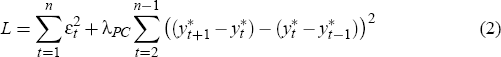
where, as in the usual H-P filter, λPC is a smoothing parameter to be chosen.[3]
2.5 Phillips Curve Specifications
To choose appropriate specifications for our Phillips curves, we adopt a general-to-specific approach. The general specification includes possible roles for lags of inflation, lagged inflation expectations from the bond market, the output gap, current and lagged changes in the gap (‘speed-limit’ terms), and current and lagged oil price and import price inflation.
In terms of the generic form of the Phillips curve, equation (1) above, the general specification assumes that inflation expectations are a linear combination of lagged inflation and inflation expectations from the bond market,
and that the vector of other variables is of the form
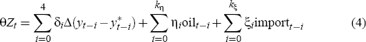
where 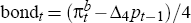 is the excess of bond market inflation expectations over
lagged year-ended inflation, expressed in per-quarter terms;
is the excess of bond market inflation expectations over
lagged year-ended inflation, expressed in per-quarter terms; 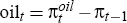 is the
excess of quarterly oil price inflation over lagged inflation; and
is the
excess of quarterly oil price inflation over lagged inflation; and 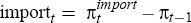 is
the excess of import price inflation over lagged inflation. For all the price series (core
consumer prices, oil prices and import prices), we use the first difference of the log price
level to approximate the quarterly inflation rate. We impose the constraint
is
the excess of import price inflation over lagged inflation. For all the price series (core
consumer prices, oil prices and import prices), we use the first difference of the log price
level to approximate the quarterly inflation rate. We impose the constraint  , to
ensure that when expected inflation,
, to
ensure that when expected inflation,  , is expressed as a linear
combination of lags of inflation and bond market inflation expectations, the coefficient weights
sum to unity. A full description of the data is provided in Appendix
D.[4]
, is expressed as a linear
combination of lags of inflation and bond market inflation expectations, the coefficient weights
sum to unity. A full description of the data is provided in Appendix
D.[4]
Australian quarterly GDP data are now available from 1959:Q3 to the present. However, 1971:Q4 is the first quarter for which we have original-vintage GDP data back to 1959:Q3, and so our real GDP vintages run from 1971:Q4 to 2001:Q4; 121 vintages in all.
For a given vintage of GDP data, we start with the general specification defined by equations (1), (3) and (4) above. The values of kα, kβ, kη, and kξ, which define the lag lengths of the variables, are kept small (most commonly, kα = 4, and kβ = kη = kξ = 2), although some searching is also undertaken of variables at longer lags (lag lengths of up to eight). Variables with coefficient t-statistics less than about 1.5 are sequentially eliminated, which leads eventually to a parsimonious specific specification. As it turns out, the coefficients on most variables in most specific specifications have t-statistics greater than 2, and the coefficient on the output gap usually has a t-statistic in excess of 5.[5]
Rather than conduct a new specification search for each new data vintage, we revisit the specific specification of the Phillips curve whenever significant deterioration is observed in the performance either of the overall equation or of its components; or, in any event, roughly every 10 to 12 years. Particular emphasis is placed on the stability of the coefficient on the output gap. In analysing coefficient stability and equation performance, we use both regressions where the start date is held fixed (at 1961:Q2) and 15-year rolling regressions.
Conducting specification searches only intermittently seems to make little difference to our estimates of potential output and the output gap, except on rare occasions when inflation is subject to a major shock of a type which has not been seen before. The chief instance of this is the first oil price shock in the early 1970s, and when such events occur, we re-specify the Phillips curve more frequently.
In all, for the 121 data vintages from 1971:Q4 to 2001:Q4, five broad Phillips curve specifications are used, as outlined in Table 1. Within the five periods delineated in Table 1, minor additional changes are also sometimes made to the Phillips curve specification for particular vintages. Full details of these re-specifications, together with a brief discussion of the reasoning behind the changes, can be found in Appendix C.
| Date of vintage | Broad equation specification |
|---|---|
| Note: Start of sample for all regressions is 1961:Q2. | |
| 1971:Q4 to 1973:Q3 | 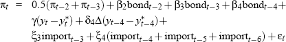 |
| 1973:Q4 to 1974:Q2 | 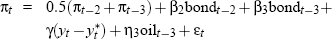 |
| 1974:Q3 to 1986:Q2 | 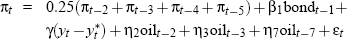 |
| 1986:Q3 to 1998:Q2 | 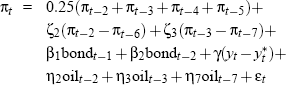 |
| 1998:Q3 to 2001:Q4 | 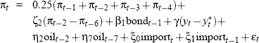 |
Footnotes
Not surprisingly, the econometric approach we employ is robust to such changes. [1]
Note that this process leads to a real-time potential output series subject to occasional substantial breaks. For example, publication after several years of a new and different estimate of the growth rate of potential output over recent history, say in response to apparent persistent under- or over-performance by the economy, leads to a sudden break in the real-time estimate of potential output at that time. [2]
We choose λPC = 80, which leads to derived potential output series that are much smoother than those derived from an H-P filter of the output data with the standard smoothing parameter of λHP = 1,600. In the notation of Laxton and Tetlow (1992), our minimisation procedure corresponds to a multivariate H-P filter of type (0,1,0,λPC). We examine the sensitivity of our results to a change in the value of λPC later in the paper. [3]
Provided  , the constraint
  does
not imply that expectations are a weighted sum of past inflation with weights that sum
to one. Our specification should not therefore be subject to Sargent's critique of
the accelerationist Phillips curve (Sargent 1971). Note also that there are some minor
aspects of the data that are not available in real time. They are discussed in Appendix D. The most substantive of them involves the
construction of bond market inflation expectations before 1993, which requires the value
of a parameter, and we use a value from Tanzi and Fanizza (1995). We establish in Appendix D, however, that our results are fairly
insensitive to the value of this parameter.
[4]
does
not imply that expectations are a weighted sum of past inflation with weights that sum
to one. Our specification should not therefore be subject to Sargent's critique of
the accelerationist Phillips curve (Sargent 1971). Note also that there are some minor
aspects of the data that are not available in real time. They are discussed in Appendix D. The most substantive of them involves the
construction of bond market inflation expectations before 1993, which requires the value
of a parameter, and we use a value from Tanzi and Fanizza (1995). We establish in Appendix D, however, that our results are fairly
insensitive to the value of this parameter.
[4]
Note that these t-statistics cannot be translated straightforwardly into levels of statistical significance because the potential output series used in the equations is generated as part of the estimation procedure, and hence the usual standard errors do not apply. It is to reduce the severity of this problem that we choose a value of the smoothness parameter, λPC, in equation (2) that leads to such smooth derived potential output series. Monte Carlo simulations on pseudo data generated by a bootstrapping procedure suggest that the coefficient estimates from our Phillips curves are not subject to significant biases (see Appendix B). [5]