RDP 2002-06: Output Gaps in Real Time: are they Reliable Enough to use for Monetary Policy? 4. Sensitivity Analysis and Confidence Intervals

In this section, we present sensitivity analysis and confidence intervals for the results derived from our preferred Phillips curve approach.

4.1 Sensitivity to Changes in the Smoothing Parameter, λ_PC

In choosing a value for the smoothness parameter, λ_PC, in equation (2), we have been guided by a desire to allow long-lived changes in the rate of potential output growth to manifest themselves, without generating high-frequency ‘noise’ in the resulting potential-output series. The value we choose, λ_PC = 80, seems to satisfy these criteria, as it generates a smooth path for potential output which nevertheless displays significant long-lived changes in its growth rate, as Figure 2 demonstrates.

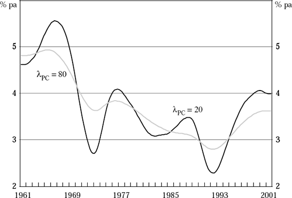
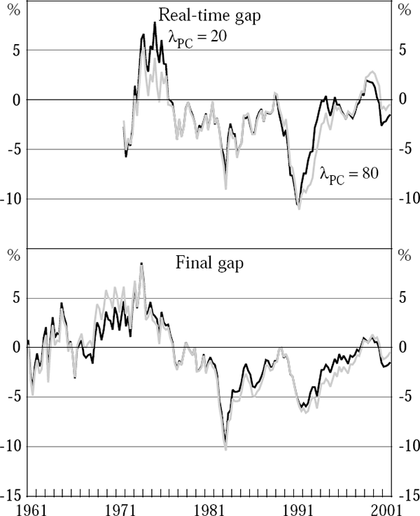
It is of interest, however, to see how sensitive our results are to this choice of parameter value. Figure 13 shows a comparison of the estimated rate of growth of potential output through time from results derived from the final vintage of data using λ_PC = 20 and λ_PC = 80. Figure 14 shows real-time output-gap estimates (upper panel) and final estimates (lower panel) assuming these alternative parameter values.^[19] Reducing the value of the parameter λ_PC to 20 generates a path for potential output growth with many more wiggles, as expected. It is striking, however, how insensitive are both the real-time and final output-gap estimates to the choice of this parameter (the root-mean-square difference between the two real-time series is 1.3 percentage points, and between the two final series, 0.7 percentage points). Over plausible ranges for λ_PC, the output-gap estimates are almost invariant to its value.^[20]

4.2 Confidence Intervals

It is also of interest to ask how large the confidence intervals are around our estimates of the output gap and the rate of growth of potential output. We use a Monte Carlo technique, summarised in Appendix B, to address these questions.

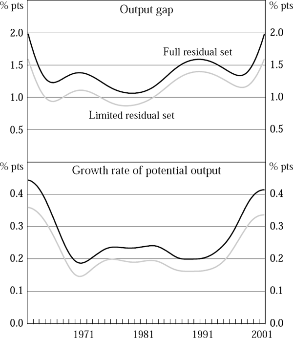
Figure 15 shows two sets of estimated standard errors for the final output gap (upper panel) and for the rate of growth of potential output (lower panel). For each line in the figure, the estimated standard errors rise considerably at each end of the sample, which is simply a manifestation of the end-point problems endemic to estimation procedures of this type. The results derived using the full set of residuals imply that the −0.5 per cent estimate of the output gap in 2001:Q4 has an associated standard error of 2.1 per cent, compared with a standard error of 1.1 per cent for output-gap estimates near the middle of the sample. The standard error of the annualised growth rate of potential output in 2001:Q4 is 0.4 per cent (the point estimate for potential growth at this time is 3.6 per cent), compared with 0.2 per cent in the middle of the sample.^[21]

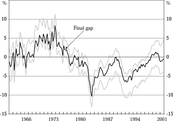
Figure 16 shows the 95 per cent confidence interval for the final output-gap estimates, based on Monte Carlo simulations using the full set of Phillips curve residuals. At this level of confidence, the results imply that the output gap is non-zero in 95 of the 163 quarters of the sample; that is, 58 per cent of the time.^[22] These results are very different from those of Orphanides and van Norden (2001), who report that, using the Gerlach-Smets approach, their final output-gap estimates for the US are virtually never significantly different from zero over the period 1966 to 1997.^[23]

Footnotes

The results assuming λ_PC = 80 are those that have been shown throughout the paper. For each data vintage, the results derived using λ_PC = 20 use the same Phillips curve specification as for the λ_PC = 80 results (that is, the specifications summarised in Table 1 and Appendix C) although the estimated parameter values in these Phillips curves would be different. [19]

It is also of interest to report how large the smoothness parameter, λ_HP, in a H-P filter of actual output needs to be to generate the same smoothness in the derived potential output series as for these values for λ_PC in our Phillips curves. We quantify ‘smoothness’ on the basis of the sum used in the loss function, equation (2), and report results for the final data vintage. To generate the same potential-output smoothness as for our Phillips curve results with λ_PC = 80, requires a value for λ_HP of about 40,000. To generate the same smoothness as for our Phillips curve results with λ_PC = 20, requires a value for λ_HP of about 1,600. [20]

When results are derived using only the post-1976 residuals, the estimated standard error of the output gap falls to 1.7 per cent in 2001:Q4, and 0.9 per cent in the middle of the sample, while for the annualised growth rate of potential output, the standard error falls to 0.3 per cent in 2001:Q4, and 0.2 per cent in the middle of the sample. All the results in Figure 15 are derived assuming our standard value λ_PC = 80. Using instead λ_PC = 20 gives standard error profiles which are very similar for the gap, but somewhat higher for the growth rate of potential output. [21]

Using the reduced set of residuals, the output gap is non-zero 66 per cent of the time, with 95 per cent confidence. Interestingly, the 95 per cent confidence interval in Figure 16 is not symmetrically distributed around the output-gap estimates derived from the actual data. [22]

It may also reflect the fact that Orphanides and van Norden's results also allow for uncertainty about the true value of the Kalman gain, the Kalman-filter equivalent of our smoothness parameter λ_PC, which is not incorporated in our confidence intervals. [23]