RDP 2002-06: Output Gaps in Real Time: are they Reliable Enough to use for Monetary Policy? 3. Results
September 2002
- Download the Paper 184KB
In this section we report on the performance of our Phillips curve method of estimating output gaps, both using the latest available data and in real time. We also compare this performance with that of alternative approaches to estimating output gaps, both for Australia and the US (as reported in Orphanides and van Norden (2001)).
Figure 1 shows some of the data used in the estimation of our Phillips curves. Included in the figure are the core consumer price inflation series we use, inflation expectations from the bond market, and oil and import price inflation. Also shown is the year-ended growth rate of GDP from the final vintage of data, the 2001:Q4 vintage, along with a 10-year moving average which shows how average GDP growth has varied over the past four decades.
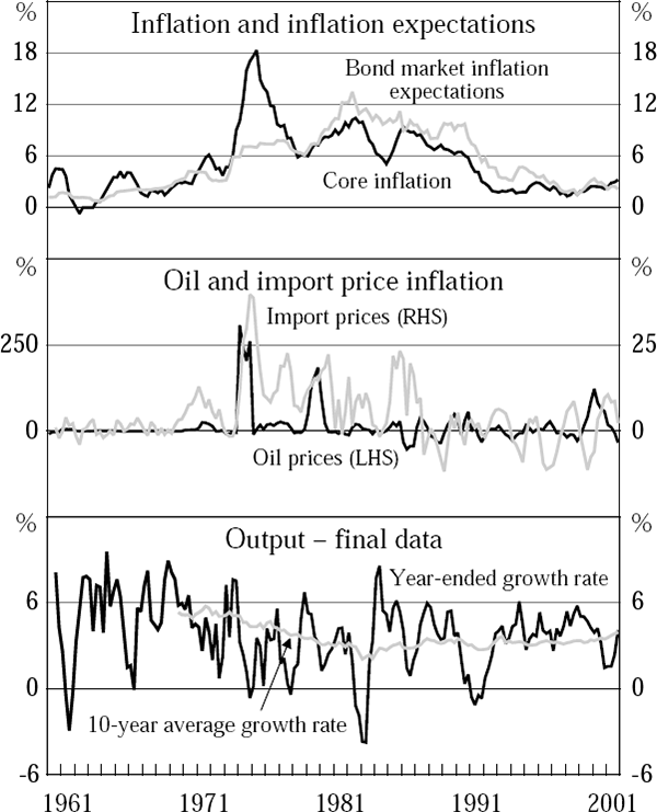
Notes: The inflation rates (core consumer price, oil, and import price) and output growth are year-ended percentage changes. The estimation results, however, use log-differences to approximate percentage changes.
3.1 Preferred Phillips Curve Method of Estimating the Output Gap
Table 2 reports estimation results for the final Phillips curve specification estimated on the final vintage of GDP data. The estimated equation explains a sizable fraction of the variation in quarterly inflation over the past four decades. The t-statistic on the output-gap coefficient, γ, is about 6. Although this t-statistic does not have a standard t-distribution, the simulations reported in Appendix B suggest that the coefficient γ is highly significant. It is also noteworthy that inflation expectations from the bond market play an important role in the equation – they contribute about 40 per cent to inflation expectations (since the coefficient on bondt−1 is about 0.4), with the remaining 60 per cent being contributed by lags of inflation – and that there is no apparent serial correlation in the equation residuals.
 |
||
|---|---|---|
| Coefficient | Value | t-statistic |
| ζ2 | 0.112 | 2.408 |
| β1 | 0.418 | 6.939 |
| γ | 0.064 | 6.081 |
| η2 | 0.007 | 3.102 |
| η7 | 0.007 | 3.324 |
| ξ0 | 0.023 | 2.202 |
| ξ1 | 0.020 | 1.845 |
| Summary statistics | Value | |
| R2 | 0.823 | |
| Adjusted R2 | 0.817 | |
| Standard error of the regression | 0.004 | |
| Breusch-Godfrey LM test for autocorrelation (p-value): | ||
| First order | 0.976 | |
| First to fourth order | 0.419 | |
Note: The sample is 1961:Q2 – 2001:Q4 (n = 163).
Eliminating the term  from the estimating equation
reduces the regression R2 (adjusted R2) to
0.78 (0.77). from the estimating equation
reduces the regression R2 (adjusted R2) to
0.78 (0.77).
|
||
Figure 2 shows estimates of the growth rate of potential output and the output gap over the past four decades based on the estimated results using the final data vintage. We refer to these output-gap estimates as the ‘final’ output-gap estimates.
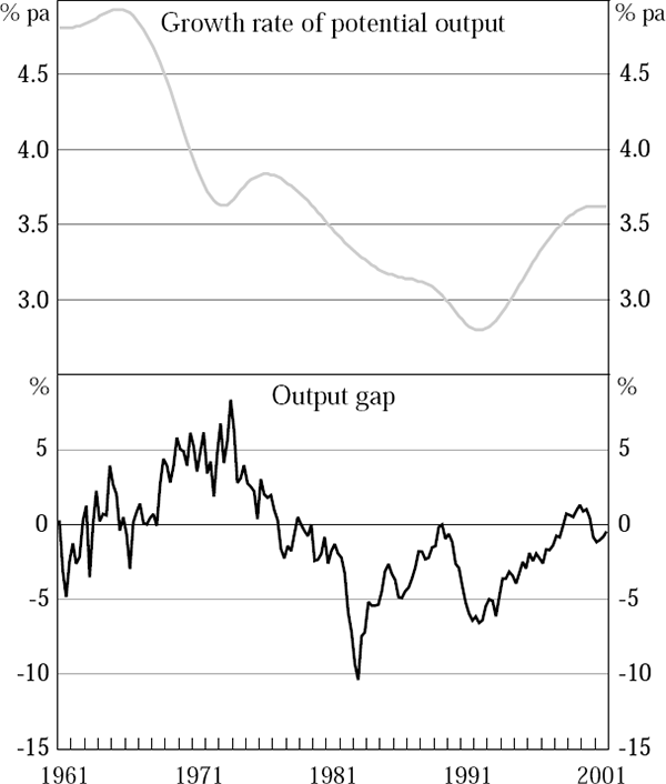
Figure 3 shows the (log) levels of actual and potential output, again based on the estimated results using the final data vintage. The smoothness of the potential output series is also clear from this figure.
The results suggest that the potential capacity of the economy grew at an annual rate of nearly 5 per cent through much of the 1960s before slowing over the next couple of decades to an annual rate more like 3 per cent in the early 1990s. In the latest few years, however, this growth rate appears to have accelerated to a little over 3.5 per cent per annum.
The estimated output gap implies that the economy was operating above its potential capacity in the last few years of the 1960s, and for much of the 1970s, and below its potential through much of the 1980s and 1990s. Not surprisingly given how they were generated, these patterns of capacity utilisation appear broadly consistent with the behaviour of inflation over the four decades.[6]
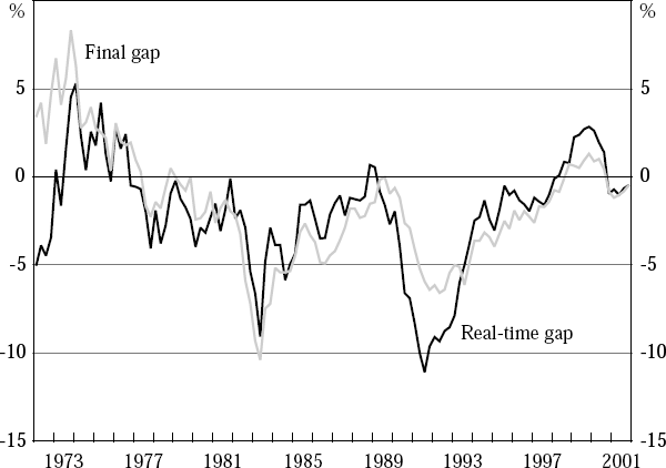
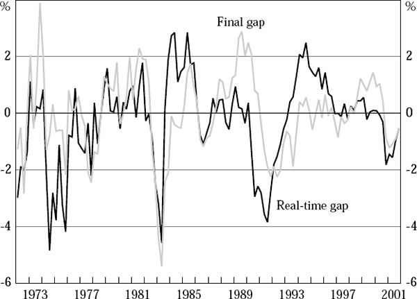
To examine the scale of the real-time problem, we construct a new series of output-gap estimates, the real-time estimates. To do so, we extract the last estimate from the output-gap series derived from each data vintage. The real-time output-gap estimates are then these last estimates, strung together into a new composite series. This real-time output gap is shown along with the final output-gap estimates in Figure 4.

The results of this exercise are quite encouraging. There is quite a close correspondence between the real-time and final estimates of the output gap for most of the past three decades, although two periods of divergence stand out – the first few years of the 1970s and the few years surrounding the early 1990s recession.[7] Before discussing these two periods, however, we present the results of a further exercise which proves illuminating.
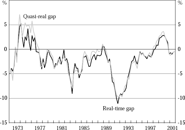
Recall that the real-time estimates of the output gap differ from the final estimates both because they use different vintages of GDP data (with the former using a different data vintage for each output-gap estimate, while the latter uses the final vintage throughout), and also because, in contrast to the final estimates, no information about the future is used in the construction of the real-time estimates. We can assess the relative importance of these two influences by constructing an alternative set of real-time estimates, the ‘quasi-real’ estimates. The quasi-real estimate of the gap in period t is constructed using the final-vintage data up to period t, rather than the period-t data vintage. Any differences between the real-time and quasi-real output-gap estimates are therefore due entirely to data revisions, since estimates in the two series at any point in time are derived using data over identical time periods.[8]
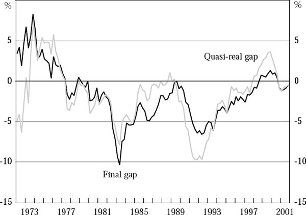
As the results shown in Figure 5 demonstrate, the real-time and quasi-real output-gap estimates are quite similar for most of the past three decades, although there are some noticeable differences in the mid 1970s.[9] It seems clear, therefore, that the predominant reason that real-time output-gap estimates differ from final estimates is not because of data revisions, but because (with the obvious exception of the last quarter in the sample) the final estimates use information about the future that is unavailable in real time.[10]
We can now return to the discussion of the two periods of divergence between the real-time and final output gaps highlighted in Figure 4 – the first few years of the 1970s and the few years surrounding the early 1990s recession – confident that the divergence is not due primarily to data revisions. Two further figures aid the discussion. Figure 6 shows the final output-gap estimates together with the quasi-real estimates, to abstract from data-revision issues. Figure 7 shows the unexplained residuals from the final Phillips curve, estimated over the whole sample, 1961:Q2 to 2001:Q4, using the final data vintage. The equation clearly does a poor job explaining inflation around these two periods of divergence, with the sample's three largest residuals in absolute value occurring in 1973:Q4, 1974:Q3 and 1991:Q1.
Note: &&&&
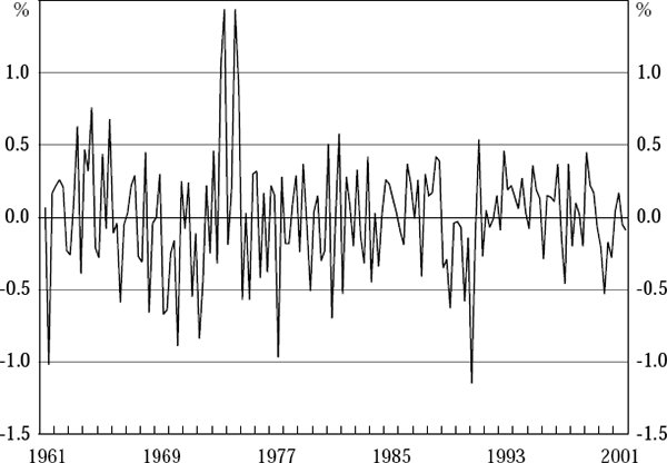
Some part of the high inflation outcomes of 1973/74 is a consequence of wage developments in the economy that should be regarded, at least to some extent, as unrelated to the state of the economy and the size of the output gap.[11] Unsurprisingly, Phillips curves estimated using either real-time or final-vintage data up to 1973 fail to anticipate this partly exogenous event. As a consequence, output gaps derived from these Phillips curves perform particularly poorly when compared with final output gaps, as Figures 4 and 6 make clear.
Given the partly exogenous nature of this event, however, we are inclined to view it as not particularly informative about general real-time problems with output-gap estimates. As a consequence, we focus much of our analysis on the 28 years after this event, that is, from 1974:Q1 to 2001:Q4.[12] Nevertheless, for completeness, we also report results for our full set of data vintages, from 1971:Q4 to 2001:Q4.
The second period of significant divergence between the real-time (or quasi-real) and final output-gap estimates occurs around the time of the early 1990s recession. Inflation fell more rapidly at that time than the average behaviour of inflation over the past four decades would lead one to expect, as is clear from the sequence of negative residuals around that time from the final estimated Phillips curve – including the largest negative residual in the sample, in 1991:Q1 (Figure 7). Phillips curves estimated using information up to that time interpret this unexpectedly rapid disinflation as a sign that the output gap is large and negative at that time – an interpretation that is subsequently revised as later information arrives. But this, of course, is simply a classic illustration of the real-time problem in action. The crucial issues are how large and how frequent are such real-time problems.
There is also a third period of divergence between the real-time (or quasi-real) and final output-gap estimates which is less pronounced, but nevertheless instructive. It occurs in the second half of the 1990s, at a time when (we would now assess that) potential output growth was accelerating from an annual rate of around 3 per cent at the beginning of the decade to above 3.5 per cent near its end (see Figure 2). We would not expect estimates of the level of potential output constructed during the transition to this faster rate of potential growth to be able fully to take it into account. As a consequence, we would expect real-time, or quasi-real, estimates of the output gap to be systematically above (more positive than) final estimates during this transition. While this pattern is clearly discernable in Figures 4 and 6, these real-time errors are, for the most part, quite moderate in size. This experience suggests that our approach to estimating output gaps in real time is reasonably robust to (at least moderate) changes in the rate of growth of potential output.
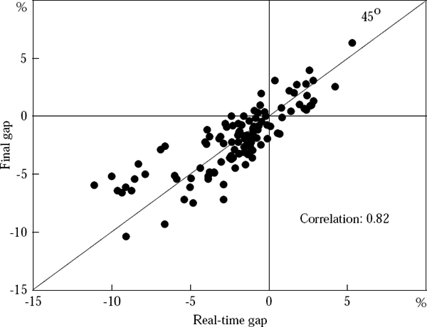
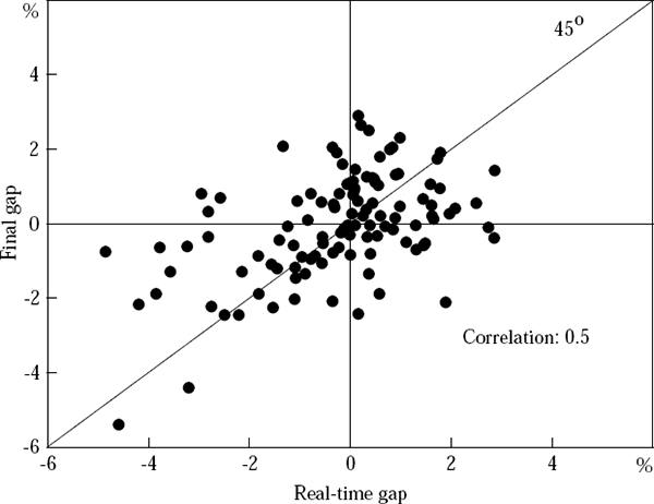
There are two further interesting ways to examine the relationship between the real-time and final output-gap estimates. One is to use a scatter-plot, as shown in Figure 8. The closeness of the relationship between the two estimates over the 28 years, 1974:Q1 to 2001:Q4, is reflected in the clustering of points relatively near the 45-degree line.
Finally, the top panel of Figure 9 shows the difference between the final and real-time output-gap estimates through time, while the subsequent panels show a decomposition of this difference, constructed so that the numbers in these lower three panels sum to the number in the top panel at each time t. The second panel shows the difference attributable to data revisions – that is, the difference between the real-time and quasi-real output-gap estimates. The third panel shows the difference between the quasi-real estimate at time t and the output-gap estimate also derived from final-vintage data up to time t, but using the final Phillips curve specification rather than the vintage-t specification used to derive the quasi-real estimates. The fourth panel of the figure shows the remaining difference.[13]
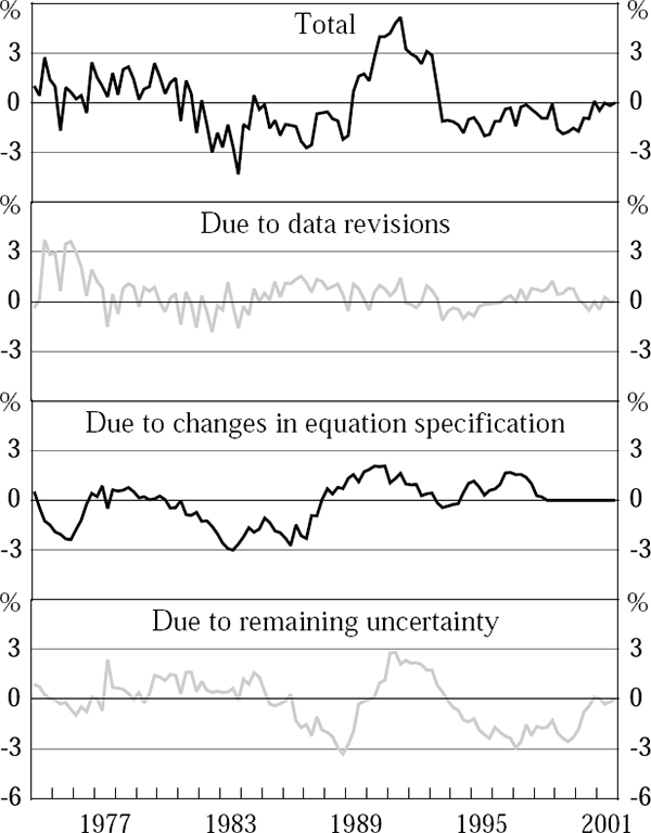
As previously discussed, data revisions generate only small changes in the output-gap estimates (panel two). Note that both panels three and four are relevant to the problem of ‘not knowing the future’. The ‘final’ specification of the Phillips curve can only be discovered after observing the economy's evolution over the full sample (relevant to panel three). Likewise, ‘final’ coefficient estimates only become clear with the full sample results (relevant to panel four).
3.2 Alternative Methods of Estimating the Output Gap
We now turn to a comparison between our preferred method of estimating real-time output gaps and alternative approaches. The alternatives we consider are two univariate methods (which assume that potential output is either a linear trend of actual output or a H-P filter of actual output) and a variant of our Phillips curve approach in which we assume that potential output grows at a constant rate, rather than allowing for changes in the growth rate as in our preferred method. (There is also a fourth alternative approach which we will discuss shortly.)
As with our preferred method, each of these alternative methods can be applied to each of the real-time data vintages, and a real-time output-gap series can then be constructed by stringing together the last output-gap estimate from each data vintage.
We can then compare each of these real-time estimates with final output-gap estimates (using the full sample of final-vintage data) derived in one of two ways: either by using the same method as for the real-time estimates (with results shown in Table 3), or by using the preferred Phillips curve method (Table 4). Table 3 also shows some of the results presented by Orphanides and van Norden (2001) for the US.
For each method, each table shows (over the relevant sample) the mean difference between the final and real-time output-gap series, the correlation between them, their root-mean-square difference (RMSD), and the first-order serial correlation of the difference (AR). Thus, for example, using a linear trend through (log) Australian output to estimate (log) potential output generates a real-time output-gap series which is on average 6.60 percentage points (ppt) below the final output-gap series derived using the same method (from Table 3). These real-time output-gap estimates can only be described as ugly. The huge differences between the real-time and final output-gap estimates using this linear-trend method occur, of course, because the growth rate of actual and potential output has been subject to significant, long-lived, changes over the four decades from the early 1960s to 2001.[14]
Applying a standard H-P filter (with λHP = 1,600) to the Australian data generates real-time output-gap estimates that differ by an average of only 0.19 ppts from the final H-P filter estimates, a huge improvement over the performance of the estimates derived from linear trends. But these H-P filter estimates are nevertheless unsatisfactory in several respects. Figure 10 shows the comparison between the real-time and final output-gap estimates derived using H-P filters, and Figure 11 shows a scatter plot of the two series (corresponding to Figures 4 and 8 for our Phillips curve method).
The relationship between the real-time and final H-P filter output-gap estimates is much less clear than between the corresponding series when they are derived using the preferred Phillips curve method, as a comparison of the relevant figures makes clear. Real-time H-P filter output-gap estimates also appear to bear almost no resemblance to our preferred final output-gap estimates – indeed, the correlation between the two series is slightly negative (see Table 4).
Furthermore, the inflation experience over the four decades from 1960 to 2001 would be particularly hard to understand on the basis of output gaps derived from the H-P filter. The average values of the final H-P filter output gaps in the four decades of the 1960s, 1970s, 1980s and 1990s, are, in percentage points, −0.1, 0.1, 0.2, and −0.1, a pattern of capacity utilisation that clearly gives no hint about the longer-run inflation developments over this time.[15]
Turning to the Phillips curve-based approach applied to Australian data, very different results emerge depending on whether or not the growth rate of potential output is allowed to vary. Assuming a constant rate of potential growth generates bad results, just at it did in the univariate case (as the results in Tables 3 and 4 make clear). By contrast, our preferred Phillips curve approach, which allows for gradual changes in the rate of potential growth, generates very substantial improvements in the performance of the real-time output-gap estimates.
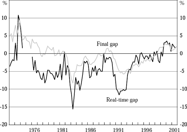
It is also instructive to examine the performance of a ‘simple’ Phillips curve. The specification we assume for this simple Phillips curve, for all data vintages, is
Results for this simple Phillips curve are derived in the same way as for the preferred Phillips curve.[16] Summary statistics are shown in the final row of Australian results in both Table 3 and 4, and a comparison of the real-time and final output-gap estimates derived using this simple Phillips curve is shown in Figure 12.
| Method | Mean Diff (ppt) | Corr | RMSD (ppt) | AR |
|---|---|---|---|---|
| Australian results | ||||
| Univariate | ||||
| Linear trend | 6.60 | 0.27 | 7.69 | 0.96 |
| H-P filter (λHP = 1,600) | 0.19 | 0.50 | 1.53 | 0.79 |
| Phillips curve-based | ||||
| Potential output growth: constant(a) | 8.44 | 0.68 | 9.68 | 0.83 |
| Potential output growth: variable | ||||
| Preferred Phillips curve method(b) | −0.01 | 0.82 | 1.81 | 0.80 |
| ‘Simple’ Phillips curve(c) | 2.86 | 0.65 | 4.23 | 0.74 |
| US results | ||||
| Univariate | ||||
| Linear trend | 4.78 | 0.89 | 5.12 | 0.91 |
| H-P filter (λHP = 1,600) | 0.30 | 0.49 | 1.83 | 0.93 |
| Phillips curve-based | ||||
| Potential output growth: | ||||
| Constant + ‘noise’ (Kuttner)(d) | 3.57 | 0.88 | 3.97 | 0.92 |
| Potential output growth: | ||||
| Variable (Gerlach-Smets)(d) | 1.64 | 0.75 | 2.17 | 0.80 |
| Notes: Results are calculated over the relevant sample of data vintages,
which is 1974:Q1–2001:Q4 for the Australian results and 1966:Q1–1997:Q4
for the US results. The US results are from Orphanides and van Norden
(2001). ‘Mean Diff’ is the mean difference between the final and
real-time output-gap series; ‘Corr’ is the correlation coefficient
between the two series; RMSD is the root-mean-square difference between them; and AR
is the the first-order serial correlation of the difference. (a) These results are derived assuming that  , where a
and b are freely estimated as part of the Phillips curve estimation for
each data vintage. The equation specifications used for these Phillips curves are
optimised in a similar way to our preferred approach. Appendix
C provides the equation specifications used for each data vintage, and
estimation results for the final data vintage. , where a
and b are freely estimated as part of the Phillips curve estimation for
each data vintage. The equation specifications used for these Phillips curves are
optimised in a similar way to our preferred approach. Appendix
C provides the equation specifications used for each data vintage, and
estimation results for the final data vintage.(b) Over the longer sample of data vintages, 1971:Q4 to 2001:Q4, Mean Diff is 0.48 ppt, Corr is 0.71, RMSD is 2.54 ppt, and AR is 0.89. (c) This Phillips curve specification is defined by equation (5) in the text. These results exclude the quarters of 1974:Q3, 1974:Q4, 1975:Q2 and 1975:Q4, in which the optimisation procedure fails to converge, or generates a negative or zero coefficient on the output gap, γ. (d) The Kuttner and Gerlach-Smets approaches use Phillips curves based solely on information about inflation and output, and use the Kalman filter to derive results. |
||||
| Method | Mean Diff (ppt) | Corr | RMSD (ppt) | AR |
|---|---|---|---|---|
|
Notes: Results are calculated over the 1974:Q1 – 2001:Q4 sample of Australian data vintages. ‘Mean Diff’ is the mean difference between the final preferred output gap series and the real-time gap series generated by the method shown; ‘Corr’ is the correlation coefficient between the two series; RMSD is the root-mean-square difference between them; and AR is the first-order serial correlation of the difference. (a) See note (c) in Table 3. |
||||
| Univariate | ||||
| Linear trend | 4.20 | 0.73 | 4.73 | 0.86 |
| H-P filter (λHP = 1,600) | −1.86 | −0.04 | 3.81 | 0.95 |
| Phillips curve-based | ||||
| Potential output growth: constant | 10.93 | 0.76 | 11.84 | 0.85 |
| Potential output growth: variable | ||||
| Preferred Phillips curve method | −0.01 | 0.82 | 1.81 | 0.80 |
| ‘Simple’ Phillips curve(a) | 1.04 | 0.55 | 3.29 | 0.19 |
Note: The real-time output gap estimates are not shown over the period 1974:Q3 to 1975:Q4 for reasons explained in note (c) in Table 3.
A comparison of the results from the preferred Phillips curve with those from this simple Phillips curve suggests that, in order to generate reasonably accurate real-time output-gap estimates, it is important to use an information-rich, and fairly well-specified, Phillips curve equation. The real-time output-gap estimates from the simple Phillips curve differ very substantially from final estimates derived either using the same method or using the preferred method (as evidenced, for example, by the large root-mean-square differences reported in the two tables).
Turning to the US results, the univariate linear-trend and H-P filter methods generate fairly poor results, just as they do when applied to the Australian data. For the Phillips curve-based approaches, the Kuttner method also seems to work poorly, just as the Phillips curve with a constant potential growth rate does for the Australian data.[17]
The Gerlach-Smets approach allows for a variable rate of potential output growth. On the basis of the Australian results, one might expect this assumption to generate a substantial improvement in performance, relative to the alternatives. There is some improvement, but nevertheless the Gerlach-Smets approach, at least when applied to US data, still seems prone to more serious real-time errors than our preferred Phillips curve approach applied to Australian data. (See, in particular, the still sizable mean difference for the Gerlach-Smets approach in Table 3.)
To some extent, the need for a richer specification for Australia is the result of it being a small, open economy so that import prices are of greater importance in modelling inflation for Australia than for the US. Nevertheless, the simplicity of the Phillips curve specification used by Gerlach-Smets may also be partly responsible for the relatively poor performance. The Gerlach-Smets Phillips curve is similar to the ‘simple’ Phillips curve defined by equation (5) above, which as we have seen, generates poor real-time output-gap estimates for Australia.[18]
Footnotes
Two factors help to explain why the output gap is negative for almost the whole of the 1980s and 1990s. First, the process of disinflation requires a negative output gap. And secondly, inflation expectations from the bond market remained above actual inflation for most of the 1980s and 1990s, as shown in Figure 1. While that remains the case, the output gap must be negative to keep inflation steady (since potential output is defined as the level of output consistent with actual inflation being equal to inflation expectations, and inflation expectations are a combination of past inflation and inflation expectations from the bond market). [6]
It is also of interest to report on the statistical properties of the real-time output-gap errors. Define the real-time output-gap estimate as equal to the final output-gap estimate plus a real-time error. Then the correlation coefficient between the final gap estimate and the error is −0.45 while the correlation coefficient between the real-time gap estimate and the error is 0.32. As argued for example by Rudebusch (2001), the first type of correlation is a measure of the amount of ‘news’ in the revisions to the output gap, while the second is a measure of the amount of ‘noise’ in the real-time estimates. The estimated correlation coefficients therefore imply elements of both. [7]
The term ‘quasi-real’ is from Orphanides and van Norden (2001). For each sample period, we construct the quasi-real output-gap estimates using the same Phillips curve specification as for the real-time estimates, though the coefficient estimates are different in general. [8]
The mid 1970s were still very early years in the production of estimates of real GDP by the Australian Bureau of Statistics. The first real GDP estimates, which were income-based, were for the 1971:Q3 vintage, while expenditure-based estimates only began with the 1974:Q4 vintage. It is perhaps not surprising, therefore, that the greatest differences between the real-time and quasi-real output-gap estimates are found in these early, experimental years. [9]
This conclusion may seem to be at odds with the results in the companion paper to this one, Stone and Wardrop (2002), which drew attention to the size of the differences between real-time and final estimates of both quarterly and year-ended output growth. The results reported here simply establish that the problem of ‘not knowing the future’ is a much more serious constraint on the reliability of real-time estimates of the output gap (as opposed to output growth) than the problem of data revisions. [10]
Australia at the time had a centralised wage-setting system in which an official body with legislated powers, the Conciliation and Arbitration Commission, set wages for much of the workforce. A left-of-centre government was elected in December 1972, coming to power for the first time for 23 years. Within a few months of the election, the Conciliation and Arbitration Commission awarded a 17.5 per cent increase in minimum wages at a time when consumer price inflation, although rising, was running at an annual rate of less than 6 per cent. Although this wage decision was undoubtedly influenced by the state of the economy at the time, it seems clear that political-economy influences also played a role. [11]
Note that focusing on the period from 1974:Q1 onwards does not exclude the effects of the first OPEC oil shock. After a period of quiescence from mid 1971 to the end of 1973, the Australian-dollar price of oil nearly quadrupled in 1974:Q1. [12]
Note that the decomposition shown in Figure 9 is not unique. To move from the real-time to the final output-gap estimates involves three changes: to the data; to the Phillips curve specification; and to the period of estimation. There is, however, some flexibility in the order in which these changes are implemented. For example, the second panel could show the difference between the real-time estimates and estimates derived using the real-time data but with the final Phillips curve specification. [13]
Not surprisingly, this method generates real-time output-gap estimates which also differ very significantly from the final estimates derived using the preferred method (see Table 4). It is interesting to note that Taylor (1993), in the paper that introduced the Taylor rule, generated estimates of the output gap by removing a linear trend from actual output. The approach arguably produced quite good estimates in that case because it was applied over a short sample of only nine years from 1984:Q1 to 1992:Q3, during which the trend rate of potential output growth was probably fairly stable. [14]
The corresponding average final output gaps using our preferred Phillips curve method in the four decades are 0.7, 2.6, −3.6 and −2.9. These decadal averages sit much more comfortably with the observed inflation outcomes – with strongly rising inflation and inflation expectations in the 1970s, and the opposite in the 1980s and 1990s. [15]
That is, for each data vintage, we find the values for γ, and the
potential output series  which minimise the loss function, equation (2), using the same smoothness parameter as
for the preferred Phillips curve, λPC = 80.
[16]
The Kuttner method assumes that potential output evolves as a random walk with constant drift (and hence potential growth differs from a constant by an i.i.d shock). This clearly introduces more flexibility into the assumed process for potential output than a linear trend, but apparently not enough. [17]
The Phillips curve specification used by Gerlach-Smets has quarterly inflation on the
left-hand side, and a constant, lagged quarterly inflation, and the output gap as
explanatory variables. This is essentially identical to our ‘simple’
Phillips curve specification, equation (5). (There is no need for a constant in our
simple Phillips curve because our optimisation procedure allows the whole potential
output series,  , to shift up or down to give a best fit to
the Phillips curve.) The only substantive difference between the two specifications is
the assumption of an MA(3) error process in the Gerlach-Smets Phillips curve. The
Gerlach-Smets approach also assumes that the output gap follows a (stationary) AR(2)
process, which would not be a good empirical description of the output gap series
derived using our preferred Phillips curve method on Australian data. It may also be
that Phillips curves in general do not explain very much of the variation in inflation
in the US (on this see Atkeson and Ohanian (2001) and Fisher, Liu and Zhou (2002)), in
which case the US example may not be a good guide to the inflation experiences of other
countries.
[18]
