RDP 2003-12: The Real-Time Forecasting Performance of Phillips Curves 4. Results
December 2003
- Download the Paper 128KB
Table 3 summarises the performance of our three main alternative approaches to forecasting inflation in real time (Phillips curve-based; AR model-based; and random walk), as well as the performance of our final vintage Phillips curve and final vintage AR model. The sample used for the forecast comparison is 1976:Q1 to 2002:Q4. Here and henceforth, dates for forecasts refer to the period for which the forecast was being made, rather than in which the forecast was being made.
| Method | Final vintage PC | Final vintage AR | Real-time PC | Real-time AR | Random walk |
|---|---|---|---|---|---|
| Forecasts for quarterly inflation (one quarter ahead) | |||||
| RMSE | 0.31 | 0.32 | 0.44 | 0.33 | 0.38 |
| Bias | 0.01 | 0.03 | −0.01 | 0.05 | 0.03 |
| Forecasts for year-ended inflation (one year ahead) | |||||
| RMSE | 0.87 | 1.16 | 1.55 | 1.23 | 1.57 |
| Bias | 0.08 | 0.16 | 0.03 | 0.33* | 0.46* |
|
Notes: Results are calculated over the forecast sample period 1976:Q1 to 2002:Q4. ‘RMSE’ is the root mean squared error between actual inflation and the series of real-time inflation forecasts generated by the method shown, in percentage points; ‘Bias’ is the average percentage point error in the forecast series over the evaluation period. * indicates that the bias is significant at the 5 per cent level. |
|||||
Note that, since we have data vintages (with corresponding real-time Phillips curves and output-gap equations) from 1971:Q4 onwards, we could in principle compare our various forecasting approaches over the longer sample 1972:Q4 to 2002:Q4 (or even 1972:Q1 to 2002:Q4, for one-quarter-ahead inflation forecasts).
One reason we do not do this is that the early to mid 1970s were a period of atypically extreme inflation volatility in Australia, partly driven by the first OPEC oil price shock in March quarter 1974. Comparisons of forecast performance which include this period thus tend to be unduly dominated by it.
A second reason is that inflation outcomes for this period were strongly influenced by decisions of Australia's then heavily centralised wage-setting system.[20] Since none of our forecasting methods are directly able to take account of these wage developments, which Gruen et al (2002) characterise as being ‘at least to some extent … unrelated to the state of the economy and the size of the output gap’ (p 16), we focus our forecast evaluation on the period from 1976:Q1 onwards.
4.1 Final Vintage Forecasting Performance
The first column of Table 3 shows that generally good inflation forecasting performance would have been achieved, over the past 27 years, by a forecaster with access, in each period, to the final vintage Phillips curve specification and historical output-gap profile, together with perfect foresight as to the future paths of the output gap, oil prices, import prices and bond market inflation expectations.[21] The root mean squared error (RMSE) achieved by such a forecaster, over the sample 1976:Q1 to 2002:Q4, would have been 0.31 percentage points for quarterly inflation one quarter ahead, and 0.87 percentage points for year-ended inflation over the coming year. This compares favourably with both our real-time AR model-based approach to forecasting inflation (RMSEs of 0.33 and 1.23 percentage points), and our random walk model (RMSEs of 0.38 and 1.57 percentage points). It also compares favourably with the performance which would have been achieved, at both the one- and four-quarter-ahead horizons, by our final vintage AR model (RMSEs of 0.32 and 1.16 percentage points).
These results for the predictive performance of our final vintage Phillips curve seem promising. The key question, however, is: does this good Phillips curve-based performance carry over from the unrealistic setting of forecasting based on our final vintage Phillips curve, to the situation we are actually interested in, out-of-sample forecasting in real time?
4.2 Real-time Forecasting Performance
Unfortunately, here the results for our Phillips curves are much less impressive. From the third column of Table 3 we see that, over the sample 1976:Q1 to 2002:Q4, our real-time Phillips curve-based inflation forecasts are unbiased, at both the one- and four-quarter-ahead horizons.[22] This accords with the findings of Orphanides and van Norden (2003) for the US, and contrasts with the bias apparent in the corresponding real-time AR model-based and random walk forecasts for inflation at the one-year-ahead horizon. Despite this bias, however, comparison of columns 3 to 5 of Table 3 shows that, in RMSE terms, both these simple, benchmark inflation forecasts perform essentially as well as, or better than, our Phillips curve-based forecasts in real time – despite the perfect foresight built into the latter in relation to variables such as oil and import prices. This is true both for one-quarter-ahead inflation forecasts, and for forecasts for inflation over the year ahead.
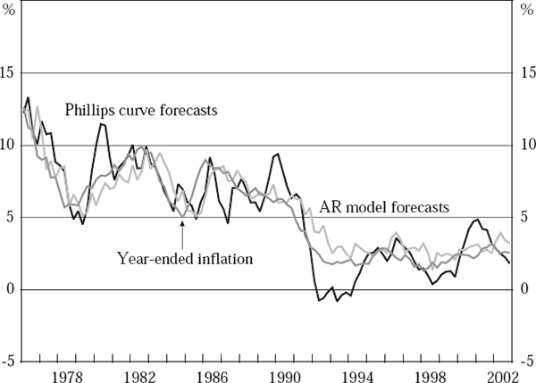
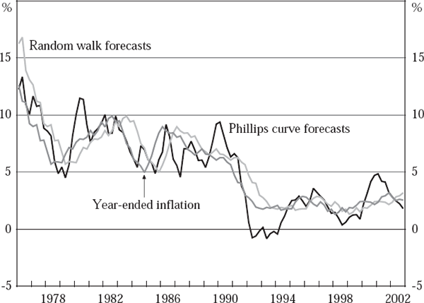
This disappointing forecasting performance in real time by our Phillips curve-based models is illustrated by Figures 1 and 2, which compare the real-time forecasts for year-ended inflation from our Phillips curve-based approach with those from our alternative benchmarks (and with actual inflation), over the sample 1976:Q1 to 2002:Q4.


These figures confirm that the large RMSEs for our Phillips curve-based inflation forecasts are mainly attributable to excessive volatility in these forecasts, rather than to forecast bias – although there are periods where our real-time Phillips curve-based forecasts for inflation persistently over- or under-shoot actual year-ended inflation, such as in the early 1990s. Interestingly, during this period of disinflation in Australia, while both of our real-time benchmark models repeatedly over-estimate inflation over the year ahead (as one would expect), our real-time Phillips curve-based forecasts are instead consistently too low for several years, starting in 1991. In part this reflects that the early 1990s is a period for which our generally reliable real-time output-gap estimates perform particularly poorly, underestimating the ‘true’ gap (as estimated on final vintage data) by around 3 percentage points for several years – see Figure 4 in Gruen et al (2002).
Figures 1 and 2 also highlight that the relative performance of our alternative, real-time approaches to forecasting inflation varies over the evaluation period. This point is further illustrated by Table 4, which breaks the RMSE results reported in Table 3 into results for five-year sub-periods – except the last, which covers only the two years from 2001:Q1 to 2002:Q4. For quarterly inflation one quarter ahead, our real-time Phillips curve-based approach outperforms our AR model-based and random walk approaches, in RMSE terms, only over the last few years (although it also achieves broadly comparable performance to our random walk forecasts in the late 1970s and early 1980s). It performs markedly worse than either real-time benchmark from the mid 1980s to the mid 1990s.
| Method | Final vintage PC | Final vintage AR | Real-time PC | Real-time AR | Random walk |
|---|---|---|---|---|---|
|
Note: ‘RMSE’ is the root mean squared error between actual inflation and the series of real-time inflation forecasts generated by the method shown, in percentage points. |
|||||
| RMSE of forecasts for quarterly inflation (one quarter ahead) | |||||
| 1976–1980 | 0.36 | 0.43 | 0.53 | 0.44 | 0.54 |
| 1981–1985 | 0.34 | 0.40 | 0.42 | 0.39 | 0.43 |
| 1986–1990 | 0.30 | 0.25 | 0.50 | 0.26 | 0.32 |
| 1991–1995 | 0.35 | 0.29 | 0.47 | 0.30 | 0.32 |
| 1996–2000 | 0.27 | 0.24 | 0.31 | 0.24 | 0.27 |
| 2001–2002 | 0.13 | 0.20 | 0.14 | 0.20 | 0.21 |
| RMSE of forecasts for year-ended inflation (one year ahead) | |||||
| 1976–1980 | 0.81 | 1.34 | 1.95 | 1.46 | 2.57 |
| 1981–1985 | 0.70 | 1.60 | 1.18 | 1.56 | 1.79 |
| 1986–1990 | 0.90 | 0.86 | 1.75 | 0.84 | 1.17 |
| 1991–1995 | 1.18 | 1.12 | 1.76 | 1.34 | 1.31 |
| 1996–2000 | 0.77 | 0.86 | 1.06 | 0.94 | 0.58 |
| 2001–2002 | 0.68 | 0.73 | 1.13 | 0.74 | 0.54 |
For year-ended inflation a similar story holds. Our real-time Phillips curve-based forecasts do better in RMSE terms than either real-time benchmark in the first half of the 1980s; and also do better than our random walk forecasts in the 1976 to 1980 sub-period. However, in all other sub-periods they do worse than either benchmark – sometimes dramatically so. For example, from 1996 onwards, a period of low and stable inflation, they perform around twice as badly in RMSE terms as our random walk forecasts (which in fact outperform all the other models considered in Table 4 over this period).
Given this generally poor performance of our Phillips curve-based forecasts in real time, it is interesting to ask: do they contain any useful additional information about future inflation, distinct from that provided by our simple alternative benchmarks? An indication that they may do comes from considering an alternative, weaker metric for measuring forecast performance, namely: how frequently does the forecast method at least predict correctly the direction of change of inflation, relative to its last value in history? In part, our interest in this metric is prompted by Fisher, Liu and Zhou (2002), who find that, for the US, Phillips curves do add some value, relative to autoregressive forecasts, by forecasting this direction of change in inflation more accurately. Table 5 shows the results for our alternative inflation forecasting models with respect to this metric.[23]
| Method | Final vintage PC | Final vintage AR | Real-time PC | Real-time AR |
|---|---|---|---|---|
| Forecasts for quarterly inflation (one quarter ahead) | ||||
| Direction correctly predicted | 67.6 | 65.7 | 62.0 | 63.9 |
| Forecasts for year-ended inflation (one year ahead) | ||||
| Direction correctly predicted | 76.9 | 63.0 | 70.4 | 62.0 |
|
Notes: Results are calculated over the sample 1976:Q1 to 2002:Q4. Results are reported in percentage terms – that is, the number of forecasts for which each method correctly predicts the direction of the change in inflation over the quarter or year ahead, as a percentage of the total number of forecasts made. |
||||
We see from Table 5 that, at least for annual inflation over the year ahead, our real-time Phillips curve-based forecasts predict the direction of the change in inflation correctly more often than do our real-time AR model-based forecasts (assessed over the full evaluation period). Indeed, they even outperform the final vintage AR model forecasts under this metric – by around 7 percentage points.
4.3 Combining Forecasts
These latter results suggest that, despite their poor performance in RMSE terms, the real-time forecasts from our Phillips curves may contain some useful information, additional to that from our benchmark models. If so, it might be possible to combine these forecasts with those from these benchmark models, to produce projections which are superior to either set in isolation. The intuition here is that, even where one set of forecasts performs much better than another, some value may be able to be gained by combining the two, if the errors in each are not perfectly correlated. We now test this possibility formally by estimating several sets of suitable ‘forecast combination’ equations.
Ex post forecast combination tests
We begin with an ex post forecast combination analysis of relative forecast performance. This involves regressing actual quarterly or year-ended inflation against two alternative forecasts for the same quantity, over our full evaluation period 1976:Q1 to 2002:Q4, and observing how much weight the regression chooses to place on each of the two competing forecasts. Specifically, for the case of quarterly inflation, let fpc denote our real-time Phillips curve-based forecasts, and let falt represent an alternative set of forecasts, either those from our realtime AR models or from our random walk benchmark (denoted far and frw respectively). Then we are interested in the weight, λ, which the regression chooses to place on fpc, relative to that placed on falt, in the regression: [24]
For year-ended inflation the corresponding regression is
where fpc and falt now denote forecasts for year-ended inflation.[25]
In all, we therefore conduct four separate ex post forecast combination tests: two for our one-quarter-ahead forecasts (real-time Phillips curve-based forecasts versus our real-time AR model-based and random walk benchmark forecasts, in turn); and another two for our one-year-ahead forecasts. The results of these regressions, estimated by OLS, are as follows:
These ex post forecast combination tests suggest that our real-time AR model-based and random walk forecasts already contain much of the information incorporated in our real-time Phillips curve-based forecasts – although not all of it. For the year-ahead forecasts especially, the Phillips curves appear to contain some information on inflation distinct from that from our AR model-based and random walk forecasts, with weights of λ = 0.36 and λ = 0.51 assigned to the Phillips curve-based forecasts in these cases.[26]
Real-time forecast combination
In the same way, however, that final vintage RMSE results do not accurately reflect the real-time, operational usefulness of a given forecasting technique, so the above forecast combination tests do not properly capture the real-time usefulness or otherwise of our Phillips curve-based forecasts, as a supplement to those from our alternative benchmark models. This is because the weights in Equations (3) to (6) are those from ex post regressions, using our various alternative real-time forecasts over the full evaluation period, 1976:Q1 to 2002:Q4. A policy-maker in the middle of this period, trying to construct optimal combined inflation forecasts in real time, would not know these optimal full-sample weights.
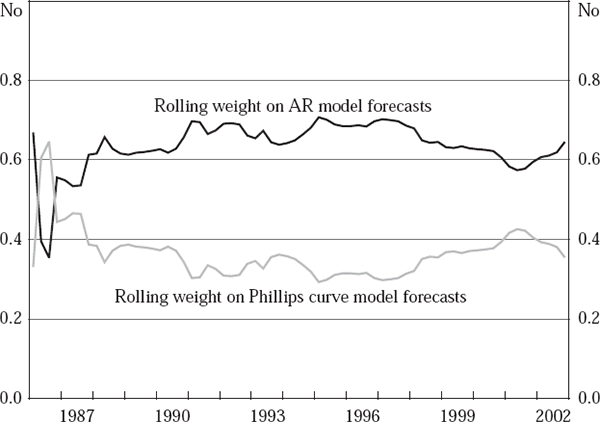
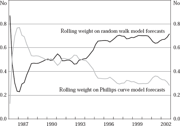
To more accurately represent the policy-maker's problem in real time, we repeat the estimation of the forecast combination equations described above (see Regressions (1) and (2)), but now on a rolling basis.[27] Specifically, we use a 10-year lagged window to determine, in each period, the weights which a policymaker would, in real time, choose to place on each of the competing forecasts for inflation. For year-ended inflation, Figure 3 shows the profile over time of the estimated real-time weights placed on our Phillips curve-based forecasts, and on our AR model-based forecasts, under this real-time approach to combining these forecasts. Figure 4 does the same for the combination of our Phillips curve-based forecasts with those from our random walk benchmark.[28]


As is evident from Figure 3, the weight placed on our Phillips curve-based forecasts for year-ended inflation, when combined in real time with our AR model-based projections, is broadly stable over time at between 29 and 43 per cent (except in the first few years of the sample). By contrast, Figure 4 shows that, when combined in real time with our random walk projections for year-ended inflation, the weight placed on our Phillips curve-based forecasts exhibits two distinct phases (again leaving aside the period of extreme volatility from 1986:Q1 to 1988:Q1). Between 1988:Q2 and 1993:Q4 this weight fluctuates narrowly between 45 and 54 per cent, before undergoing a downward shift during 1994. Thereafter, it is again fairly stable, ranging now between 28 and 38 per cent.[29]
Using the weights shown in Figures 3 and 4 also yields new series of real-time, combined, out-of-sample forecasts for inflation, over the truncated evaluation period 1986:Q1 to 2002:Q4. The relative performance of these forecasts is summarised in Table 6, from which several interesting results emerge.
| Method | Real-time PC |
Real-time AR |
Random walk |
Combined PC and AR |
Combined PC and RW |
|---|---|---|---|---|---|
| Forecasts for quarterly inflation (one quarter ahead) | |||||
| RMSE | 0.41 | 0.26 | 0.30 | 0.26 | 0.29 |
| Bias | −0.04 | 0.09* | 0.02 | 0.04 | 0.07* |
| Forecasts for year-ended inflation (one year ahead) | |||||
| RMSE | 1.51 | 1.03 | 1.02 | 0.90 | 0.97 |
| Bias | −0.20 | 0.58* | 0.26* | 0.32* | −0.04 |
|
Notes: Results are calculated over the forecast sample period 1986:Q1 to 2002:Q4. ‘RMSE’ is the root mean squared error between actual inflation and the series of real-time inflation forecasts generated by the method shown, in percentage points; ‘Bias’ is the average percentage point error in the forecast series over the evaluation period. * indicates that the bias is significant at the 5 per cent level. |
|||||
First, before even turning to the combined forecasts, it is notable that our real-time AR model-based forecasts for year-ended inflation are considerably more biased (58 basis points) over the sample considered in Table 6, than they are over the longer evaluation period considered in Table 3 (33 basis points). The reverse, however, is true for our random walk forecasts, whose bias declines from 46 to 26 basis points over the shorter sub-sample. Both methods display lower forecast RMSE over the shorter sub-sample, consistent with the period from 1976 to 1985 having been a more difficult period for which to forecast inflation than the post-1985 period.
Secondly, combining our real-time Phillips curve-based forecasts with those from our real-time AR models does generate improved forecasts, measured relative to our real-time Phillips curve-based ones alone. This improvement is evident at both the one-quarter and one-year-ahead horizons. However, relative to our real-time AR model-based forecasts, the improvement in performance of these combined forecasts is less striking. No reduction in forecast RMSE is achieved at the one-quarter-ahead horizon; and, although there is some improvement for the year-ahead forecasts, it is still fairly small (around 13 basis points). The combining process does, however, reduce the forecast bias problem present in the AR model-based forecasts since the mid 1980s – from 58 to 32 basis points.
A similar picture emerges for the forecasts obtained by combining our real-time Phillips curve-based projections with those from our random walk benchmark. Overall, these results confirm our earlier intuition that, while our Phillips curves do seem to add some power to our capacity to forecast inflation, relative to simple alternative models, the extra information they provide is only modest.
Footnotes
During this period Australia had an official body with legislated powers, the Conciliation and Arbitration Commission, which set wages for much of the workforce. In early 1973, following a change of government, the Commission awarded a 17.5 per cent increase in minimum wages, at a time when consumer price inflation, although rising, was running at an annual rate of less than 6 per cent. Further large award/minimum wage rises were mandated in May and December 1974. While wages in Australia in subsequent years were also affected by frequent Commission decisions – see Appendix A of Gruen et al (1999) – increases in average weekly earnings over these years did not again approach the extremes which occurred during 1973 and 1974. [20]
There is, of course, some circularity in this finding since, as described in Gruen et al (2002), the final vintage output-gap profile is conditioned on information about inflation over the full sample from 1961:Q2 to 2002:Q4. Hence, ‘forecasts’ generated using this gap have some information about future inflation already built into them. This circularity, however, does not apply to our real-time Phillips curve-based forecasts, since the gap estimates used in generating these forecasts in each period are conditioned only on historical inflation data, not on information about future inflation. [21]
To formally test that the one-quarter-ahead forecasts are, on average, correct, we simply regress the forecast error series against a constant (Holden and Peel 1990); while for the four-quarter-ahead forecasts, we also allow up to a third-order moving-average process in the corresponding regression (Diebold and Lopez 1996), to capture that the four-quarter-ahead forecasts actually reflect a path of forecasts for each quarter from the beginning of the forecast horizon. [22]
We exclude our random walk model from this analysis, since by definition it never forecasts inflation to change direction over the forecast horizon. [23]
Chong and Hendry (1986) refer to such a regression as an ‘encompassing test’. If λ = 1 then the first set of forecasts are said to encompass the second, which add no additional information; if λ = 0 then the opposite conclusion holds. If 0 < λ < 1 then neither model encompasses the other, and Chong and Hendry argue that this indicates that one should adapt one of the models, building into it elements from the other, until it does fully encompass the latter. However, there are obstacles to our proceeding in this way in the current setting, partly stemming from real-time considerations. See Appendix C for further details. [24]
Regressions (1) and (2) incorporate a number of implicit restrictions, such as that the weights on the competing sets of forecasts in each case sum to one. See Footnote 27 for a discussion, in the setting of real-time forecast combination, of the impact of relaxing these restrictions. [25]
If we were to treat the forecasts fpc, far and frw in Regressions (3) to (6) as exogenous, then in each case the weight on the Phillips curve-based forecasts would, in fact, be significantly different from 0 at the 5 per cent level. However, these series represent constructed data which are subject to uncertainty – stemming, for example, from errors in coefficient estimation in the models used to produce them. Hence, OLS standard errors are not valid here: see West (2000). [26]
We also considered a wide range of variations to Equations (1) and (2), for the general form of our combining equations. Alternatives considered included: relaxing the constraint that the weights on the two sets of competing forecasts sum to one; allowing a constant in the regressions; and allowing for the possibility in Regression (2) that the errors εt follow a moving average process (Diebold and Lopez 1996). These alternatives were considered both separately and jointly. None of these variations, however, yielded any significant improvement in out-of-sample combined forecast accuracy (judged in RMSE terms), either for the combination of our Phillips curve and AR model-based forecasts, or our Phillips curve and random walk forecasts. [27]
Note that Figures 3 and 4 cover the truncated evaluation period 1986:Q1 to 2002:Q4, reflecting that our use of rolling regressions to determine the combining weights in each period means that we lose 10 years from the sample for which our real-time combined forecasts are available. [28]
The chief reason for the decline over 1994 is that 1983 was a year for which our real-time Phillips curve-based forecasts perform extremely well, whereas our random walk forecasts perform rather poorly (see Figure 2). Hence, as 1983 gradually drops out of the 10-year rolling window used to estimate this weight, which occurs over the course of 1994 in Figure 4, our Phillips curve-based forecasts are assessed to lose a good deal of their value as a guide to future inflation, relative to our random walk benchmark. [29]


