RDP 2009-01: Currency Misalignments and Optimal Monetary Policy: A Re-examination 8. Optimal Policy under LCP

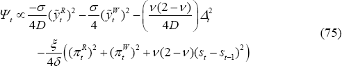
The transformed loss function, –Ψ_t, can be written as:

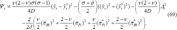
The loss function is similar to the one under PCP. The main point to highlight is that squared deviations from the law of one price matter for welfare, as well as output gaps and inflation rates. Deviations from the law of one price are distortionary and are a separate source of loss in the LCP model.

The policy-maker under discretion seeks to minimise the loss subject to the constraints of the Phillips curves, (57)–(58) and (59)–(60). There is an additional constraint in the LCP model. Note that π_Ft − π_Ht = s_t − s_t−1. But Equation (31) implies:

Using Equation (70) in conjunction with Equations (57) and (60), the following constraint can be derived:

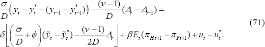
This constraint arises in the LCP model but not in the PCP model, precisely because import prices are sticky and subject to a Calvo price adjustment mechanism, rather than free to respond via nominal exchange rate changes.

Another contrast with the PCP model is that there are four sticky prices in the LCP model, so non-zero inflation rates for each of the four matter for welfare. Indeed, note that Ψ_t can be rewritten as:

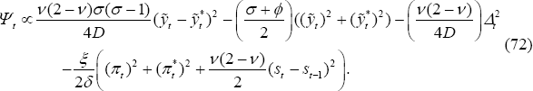
Under this formulation, the loss function is seen to depend on the aggregate CPI inflation rates, π_t and , and the change in the terms of trade, s_t − s_t−1, rather than the four individual inflation rates given in Equation (69). This formulation is particularly useful when considering a simplification below, under which s_t − s_t−1 is independent of policy.

The LCP optimisation problem under discretion becomes very complex and difficult because of the additional constraint given by Equation (71). That is because there now are endogenous state variables – the choices of home output gap relative to the foreign output gap, and the deviation from the law of one price puts constraints on the evolution of future output gaps, inflation rates and deviations from the law of one price. In the LCP case, the dynamic game between current and future policy-makers is non-trivial.

But inspection of Equation (71) reveals a special case in which the policy decision under uncertainty can be settled under the same simple conditions as in the PCP model. When ϕ = 0 – utility is linear in labour – Equation (71) simplifies considerably. Indeed, it can be rewritten as:

With ϕ = 0, we have 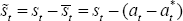. So we can write (73) as a second-order expectational difference equation:

where .

The point here is that Equation (74) determines the evolution of s_t independent of policy choices. So while s_t is a state variable, it is not endogenous for the policy-maker. One nice thing about considering this special case is that the parameter ϕ does not appear in either the target criteria or the optimal interest rate rule in the CGG model, so the targeting and instrument rules under PCP can be compared directly to the LCP model. We also note that Devereux and Engel (2003) make the same assumption on preferences.

The first-order conditions for the policy-maker can be derived independently of any assumption about the stochastic process for s_t. Equation (71) is replaced by Equation (31), expressed in ‘gap’ form, as a constraint on the choice of optimal values by the policy-maker.

In fact, in this case the policy problem can be simplified further by using the version of the loss function given by Equation (72). A useful way to rewrite (72) when ϕ = 0 is:

where the R superscript represents home relative to foreign. That is, , , etc. Likewise, the W superscript refers to the sum of home and foreign variables: 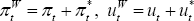, etc. Since s_t − s_t−1 is independent of policy, the policy-maker's problem can be expressed as choosing relative and world output gaps, and , relative and world CPI inflation rates, and , and the currency misalignment, Δ_t to maximise Equation (75) subject to the ‘gap’ version of Equation (31) and the linear combination of the Phillips curves that provide equations for CPI inflation in each country (which are derived here under the assumption that ϕ = 0):

The first condition seems quite similar to the first condition in the PCP case, Equation (66):

This condition calls for a trade-off between the world output gap and the world inflation rate, just as in the PCP case. But there is a key difference – here in the LCP model, it is the CPI, not the PPI, inflation rates that enter into the policy-maker's trade-off.

The second condition can be written as:

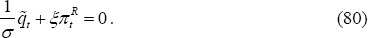
Here, q_t is the consumption real exchange rate, defined as:

is the deviation of the real exchange rate from its efficient level, where the following relationship has been used:

Equation (80) represents the second of the target criteria as a trade-off between misaligned real exchange rates and relative CPI inflation rates. In the LCP model, where exchange rate misalignments are possible, Equation (82) highlights that optimal policy involves trading off relative output gaps, relative CPI inflation rates, and the currency misalignment.

8.1 Optimal Policy under PCP versus LCP

It is helpful to compare the target criteria under PCP (Conditions (66) and (67)) and LCP (Conditions (79) and (80)).

First, compare Equation (66) to (79). Both involve a trade-off between the world output gap and world inflation. But under PCP, producer price inflation appears in the trade-off. However, world producer price inflation is equal to world consumer price inflation under PCP. To see this,

The second equality holds because the relative prices are equal in home and foreign under PCP (and, for that matter, to a first-order approximation under LCP) so .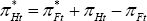

This trade-off is the exact analogy to the closed economy trade-off between the output gap and inflation, and the intuition of that trade-off is well understood. On the one hand, with asynchronised price setting, inflation leads to misalignment of relative prices, so any non-zero level of inflation is distortionary. On the other hand, because the monopoly power of labour is time-varying due to the time-varying elasticity of labour demand, output levels can be inefficiently low or high even when inflation is zero. Conditions (66) or (79) describe the terms of that trade-off. Inflation is more costly the higher is the elasticity of substitution among varieties of goods, ξ, because a higher elasticity will imply greater resource misallocation when there is inflation.

The difference in optimal policy under PCP versus LCP comes in the comparison of Condition (67) with (80). Under PCP, optimal policy trades off home relative to foreign output gaps with home relative to foreign PPI inflation. Under LCP, the trade-off is between the real exchange rate and home relative to foreign CPI inflation.

First, it is helpful to consider Equation (80) when the two economies are closed, so that ν = 2. Using (82), under this condition, D = 1, and (80) reduces to . Of course, when v = 2, there is no difference between PPI and CPI inflation, and so in this special case the optimal policies under LCP and PCP are identical. That is nothing more than reassuring, since the distinction between PCP and LCP should not matter when the economies are closed.

When ν ≠ 2, understanding these conditions is more subtle. It helps to consider the case of no home bias in preferences, so ν = 1. Imagine that inflation rates were zero, so that there is no misallocation of labour within each country. Further, imagine that the world output gap is zero. There are still two possible distortions. First, relative home to foreign output may not be at the efficient level. Second, even if output levels are efficient, the allocation of output to home and foreign households may be inefficient if there are currency misalignments.

When ν = 1, it follows from Equations (26) and (27) that relative output levels are determined only by the terms of trade. We have . On the other hand, from Equation (28) when ν = 1, relative consumption is misaligned when there are currency misalignments, . Moreover, when ν = 1, the deviation of the real exchange rate from its inefficient level is entirely due to the currency misalignment: .

Under PCP, the law of one price holds continuously, so there is no currency misalignment. In that case, Δ_t = 0, and relative home to foreign consumption is efficient. In that case, policy can influence the terms of trade in order to achieve the optimal trade-off between relative output gaps and relative inflation, as expressed in Equation (67). Policy can control the terms of trade under PCP because the terms of trade can adjust instantaneously and completely through nominal exchange rate adjustment. That is, . While and p_Ht do not adjust freely, movements in the nominal exchange rate e_t are unrestricted, so the terms of trade adjust freely.

Under LCP, the nominal exchange rate does not directly influence the consumer prices of home to foreign goods in either country. For example, in the home country, s_t = p_Ft − p_Ht. Because prices are set in local currencies, neither p_Ft and p_Ht adjust freely to shocks. In fact, as I have shown, when utility is linear in labour (ϕ = 0) monetary policy has no control over the internal relative prices.

But under LCP, there are currency misalignments, and monetary policy can influence those. Recall from (25) , so the currency misalignment can adjust instantaneously with nominal exchange rate movements. Because policy cannot influence the relative output distortion (when ν = 1) but can influence the relative consumption distortion, the optimal policy puts full weight on the currency misalignment. When ν = 1, Equation (80) can be written as When Δ_t > 0, so that the home currency is undervalued, and , so home CPI inflation exceeds foreign, the implications for policy are obvious. Home monetary policy must tighten relative to foreign. But the more interesting case to consider is when home inflation is running high, so that , but the currency is overvalued, so that Δ_t < 0. Then Equation (80) implies that the goals of maintaining low inflation and a correctly valued currency are in conflict. Policies that improve the inflation situation may exacerbate the currency misalignment (implying an even larger correction of e at some future date). Equation (80) parameterises the trade-off.