RDP 2009-01: Currency Misalignments and Optimal Monetary Policy: A Re-examination Appendix B: Welfare Functions and Other Derivations
March 2009
- Download the Paper 512KB
B.1 Derivation of Welfare Function in Clarida-Galí-Gertler Model with Home Bias in Preferences
The object is to rewrite the welfare function, which is defined in terms of home and foreign consumption and labour effort, into terms of the squared output gap and squared inflation. The joint welfare function of home and foreign households is derived, since cooperative monetary policy is being examined.
Most of the derivation requires only first-order approximations of the equations
of the model, but in a few places, second-order approximations are needed.
If the approximation is first-order, the notation  is used to indicate that there are second-order and higher terms left out, and if
the approximation is second-order,
  is used. (a
is notation for the log of the productivity shock.)
From Equation (1) in the text, the period utility of the planner is given by:
Take a second-order log approximation around the non-stochastic steady state. Allocations
are assumed to be efficient in steady state, so  .
The fact that
  follows from the fact that in steady state
C = N from market clearing and symmetry, and
  from the condition
that the marginal rate of substitution between leisure and consumption equals
one in an efficient non-stochastic steady state.
It follows that:
Since maximising an affine transformation of Equation (B2) is equivalent, it is convenient to simplify that equation to get:
Utility is maximised when consumption and employment take on their efficient values:
In general, this maximum may not be attainable because of distortions. Writing  ,
where
  ,
it follows that:
or
The object is to write (B6) as a function of squared output gaps and squared inflation
if possible. A second-order approximation of  is needed. But for the rest of the terms, since they are squares and products, the
first-order approximations that have already been derived will be sufficient.
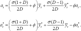
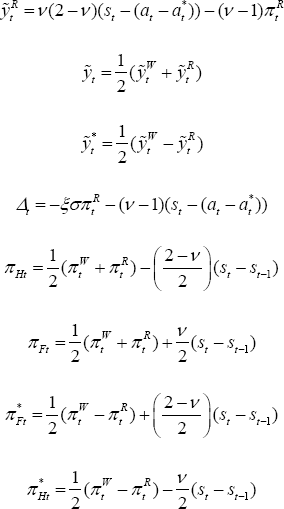
Recalling that Δt = 0 in the PCP model, Equations (A7)–(A8) can be written as:
where  .
.
It follows from (B7) and (B8) that:
Next, it is easy to show that:
These follow as in Equations (A2)–(A3) because  and
and  (and similarly in the foreign country).
Expressions for  and
and  are required. From Equations (A10)–(A11):
Using  and
and  ,
these can be written as
Turning attention back to the loss function in Equation (B6), focus first on the
terms  .
.
As noted above, these involve only squares and cross-products of  ,
and
,
and  .
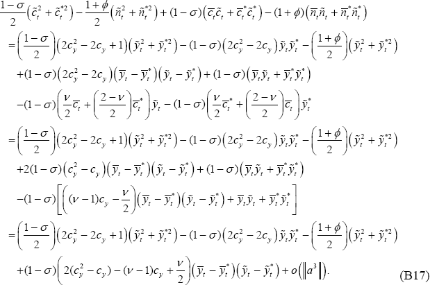
Equations (B9)–(B16) can be substituted into this expression. It is
useful to provide a few lines of algebra since it is a bit messy:
Now return to the  term in Equation (B6) and conduct a second-order approximation. Start with Equation
(18), dropping the k−1 term because it will not
affect the approximation, and noting that in the PCP model,
  :
:
Then use Equation (22), but using the fact that  and there are no deviations from the law of one price:
Substitute in to get:
Solve for Ct:
Take first and second derivatives, evaluated at the non-stochastic steady state:
Then this second-order approximation is obtained:
Symmetrically,
Since only  is of interest, these can be added together to get:
Now take a first-order approximation for st to substitute out for  . Equation (A9) implies:
Substituting into Equation (B28) leads to:
where  .
.
Evaluating (B29) at flexible prices:
It follows from the fact that  that
that
See Section B.3 below for the second-order
approximations for  and
and  :
:
Substitute expressions (B31)–(B33) along with (B17) into the loss function (B6):
Some tedious algebra demonstrates that
So, finally it is possible to write:
This expression reduces to CGG's when there is no home bias (γ = 1). To see this from their expression at the top of p 903, multiply their utility by 2 (since they take average utility), and set their γ equal to ½ (so their country sizes are equal).
B.2 Derivation of Welfare Function under LCP with Home Bias in Preferences
The second-order approximation to welfare in terms of logs of consumption and employment of course does not change, so Equation (B6) still holds. As before, the derivation is broken down into two parts. First-order approximations to structural equations are used to derive an approximation to the quadratic term
Then second-order approximations to the structural equations are used to derive an
expression for  .
.
The quadratic term involves squares and cross-products of  and
and  .
Expressions (B9)–(B10) still provide first-order approximations for
 and
and  ;
Equations (B13)–(B14) are first-order approximations for ñt
and
  ;
and Equations (B15)–(B16) are first-order approximations for
  and
and  . But Equations (A7)–(A8)
and (B11)–(B12) are required to derive:
With these equations, the derivation as in Equation (B17) can be followed. After
tedious algebra, the same result is achieved, with the addition of the terms
 and
and  .
Note that the last term involves output levels, not output gaps. That is:
The derivation of  is similar to the PCP model. However, one tedious aspect of the derivation is that
the equality
  , that holds under PCP and flexible prices,
cannot be used. The equilibrium conditions are expressed for home output,
and its foreign equivalent, from Equations (18) and (19):
Directly taking second-order approximations of these equations around the efficient non-stochastic steady state implies:
Note that in a second-order approximation,  cannot be imposed. However,
  can be imposed. Then adding Equations (B42)
and (B43) together, leads to:
Next, Equations (A7), (A8) and (A9) can be used to get approximations for  and
and  .
These equations are linear approximations for
  and st,
but since the goal is to approximate the squares of these variables, that
is sufficient. With some algebra, it can be shown that:
Then, substituting Equation (B45) into Equation (B44) and rearranging, it follows that:
Note that if Δt = 0, Equation (B46) leads to the second-order
approximation for  from the PCP model.
Then following the derivations as in the PCP model derivation of Equation (B31), it follows that:
As shown in Section B.3, the following second-order approximation can be made:
Equation (B47) and (B48), along with Equation (B39), can be substituted into the
loss function (B6). Notice the cancellations that occur. The cross-product
terms on  in Equations (B39) and (B47) cancel. The other cross-product terms involving output
gaps and efficient levels of output also cancel, just as in the PCP model,
when Equation (B35) was used. Hence:
B.3 Derivations of Price Dispersion Terms in Loss Functions
In the PCP case, it is true that
where  df. Taking logs:
It is the case that  ,
,
where we define
Following Galí (2008), note that
By the definition of the price index  .
Hence, from (B53),
It is also the case that
It follows, using (B54):
Note the following relationship:
Using our notation for variances,  ≡ var(pHt), and taking the log of (B56) leads to
Substituting this into Equation (B51), and recalling that  ,
implies Equation (B32). The derivation of Equation (B33) for the foreign country
proceeds identically.
For the LCP model, the following second-order approximation to the equation  is used:
In the LCP model, it is possible to write:
where the definitions of VHt and  are analogous to that of Vt
in the PCP model. Taking a second-order log approximation to the Expression (B60):
The same steps as in the PCP model can be followed to conclude:
Substituting these expressions into Equation (B61) and cancelling higher-order terms, implies:
Then using Equation (B59), this implies that:
Keeping in mind that  :
:
Following analogous steps for the foreign country,
Adding Equations (B66) and (B67) gives Equation (B48).
Finally, to derive the loss functions for policy-makers (Equation (65) for the PCP
model and (69) for the LCP model), note that the loss function is the present
expected discounted value of the period loss functions derived here (Equation
(B36) for the PCP model and (B49) for the LCP model). That is, the policy-maker
seeks to minimise  .
.
Following Woodford (2003, Chapter 6), it can be seen that, in the PCP model, if prices are adjusted according to the Calvo price mechanism given by Equation (50) for PHt, then
Analogous relationships hold for  in the PCP model, and for
  , and
, and  in the LCP model.
This relationship can then be substituted into the present value loss function,
 ,
to derive the loss functions of the two models presented in the text.
B.4 Solutions for Endogenous Variables under Optimal Policy Rules
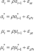
Assume that shocks follow the processes (where the W superscript on the wage mark-up shocks have been dropped):
st is determined by:
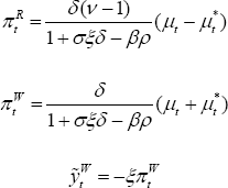
The solutions for the variables that appear in the loss function under the optimal policy described in the text are:


